Prosjektoppgave:
Dynamisk posisjonering av fartřy ("DP")
Introduction
Dynamic positioning means position control of vessels using thrusters and propellers as actuators to keep the vessel at a reference position relative to the seafloor or relative to another vessel or sea platform. DP is an important technology in sea operations.
What this project is about
In this project you will design and simulate a simplified DP system in LabVIEW. The system includes a Kalman Filter for estimation of one of the environmental forces acting on the vessel. This estimate is used in the model based position controller.
Software
- LabVIEW with Control Design Toolkit and Simulation Module
Technical information about DP
The following figures and mathematical expressions are from documentation produced by the Norwegian company Kongberg Maritime (KM). (KM is one of the world's leading producers of DP systems.) KM has approved using the information presented in this document for teaching purposes.
Figure 1 shows the main components in a DP system.
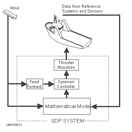
Figur 1. (Kilde: Kongsberg Maritime)
Figure 2 shows a vessel with definitions of the vessel-fixed coordinates surge, sway and yaw.
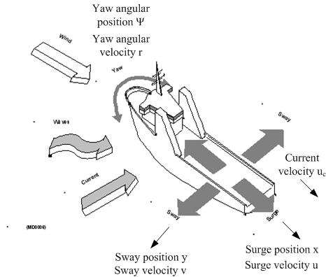
Figur 2. (Kilde: Kongsberg Maritime)
Figure 3 shows the relation between the earth-fixed coordinate system and the vessel-fixed coordinate system.
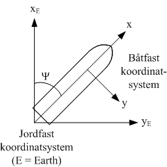
Figur 3
Below is a simplified model of a vessel. The model is based on force balances along the surge axis and the sway axis, and torque balance about the yaw axis (rotation). (The nomenclature is according to Kongsberg Maritme.)
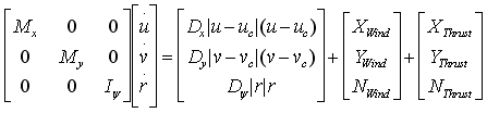
X and Y are forces. N is torque. Sub-index c means water current. M is mass. I is inertia. D is damping coefficient. The first vector at the right side of the the equality sign are hydrodynamic forces or torque.
Although they is not needed in the tasks in this project, the coordinate transformations from vessel-fixed velocities to earth-fixed velocities are presented here:
![]()
For simplicity, this project considers only surge movement, assuming there is no movement in the other directions.
The following information applies for a given vessel:
- Vessel length is Lpp = 233 m. Width is 42 m. Depth is 10 m. (However, these parameters are not needed in this project.)
- Mx = 71164 tons
- Dx = -8.4 kN/(m/s*m/s).
- uc typically varies in the range 0 - 3 m/s.
- The longitudal thruster force XThrust (which is the actuator force) has a limit of 552 kN forwards and 467 kN backwards.
- Longitudal wind force (in the surge direction) is
XWind = Vw2[cWx1 cos(fi) + cWx2 cos(3fi)]
where Vw is the wind speed relative to the vessel. fi is wind angle relative to the vessel. If the wind comes from the front (of the vessel) fi = 180 degrees. cWx1 = 0.1838 and cWx2 = -0.0068 are so-called first and second order wind coefficients. One example: With Vw = 20 m/s and fi=180 deg, we have XWind = -70.8 kN.
Figure 4 shows the definitions of the different wind forces.
Figur 4: Vindstyrker
- uc varierer typisk i omrĺdet 0 - 3 m/s. (uc skal estimeres med Kalmanfilter.)
- Langskips propellkraft XThrust (pĺdraget pĺ fartřyet) har en begrensning pĺ 552 kN forover og 467 kN bakover.
- Til info (trengs ikke i oppgaven): Fartřyets lengde er Lpp = 233 meter. Bredden er 42 meter. Dypgang er 10 meter.
Comment: With "DP" terminology the unit "ton" represents a force of 1kN, but in this project tons represents 1000kg, as normal.
Tasks
The simulation time step can be set to 1 second, and you may run the simulator 100 times faster than real time.
Tip: Use the units consequently, for example use N as force unit everywhere in the simulator.
- Implement a simulator containing the following:
- The vessel model of the movements along the surge axis. All parameters
should be available at the front panel of the simulator (including vessel
parameters and wind model).
Check that the simulator shows a correct response, for example by comparing simulated velocity and manually calculated velocity under static conditions.
- A Kalman Filter (the predictor-corrector version) based on the
following:
- The position is x1 is measured.
- The wind angle and speed have known values, because they are assumed to be measured.
- The water current speed uc is assumed to be constant or slowly varying, but it is not measured, so you must estimate it with the Kalman Filter. Hint: Augment the ship model with a differential equation describing the assumed (modelled) behaviour of the the water current.
- Use a steady-state Kalman Filter gain, Ks. You can
calculate Ks from a linear vessel model based in linearization
about the present operating point. You can calculate Ks with the Kalman Gain
function (Ks is the M-output from this function).
Use the Observability Matrix-function to check if the system is observable in this operating point. Note: The system is non-observable in the particular "zero-operating point" where the difference between the vessel speed and the water current is zero, and therefore you must use a linear model corresponding to a non-zero speed difference when calculating Ks.
Note: The Kalman Gain function can be used in 4 different ways, denoted "instances" in the LabVIEW Help about this function. You should use the CD Kalman Gain (Deterministic) instance.
Hint: The calculation of Ks can be implemented outside the Simulation Loop, in a While Loop with a relatively large cycle time.
Hint: Your LabVIEW program may look quite similar to the one described in Example 19 on page 112 etc. in the compendium. In one of the figures in this example it is shown how you can define a state-space model using a combination of a Formula node and the CD Create State-Space Model function. The Model output from this function can then be connected to the Model input on the Kalman Gain function. - You should implement the Kalman Filter equations in a Formula Node in LabVIEW.
- Check that the Kalman Filter produces a correct estimate of the water
current (by comparing the estimate with the value that you adjust on the
front panel).
-
A positional control system for the vessel based on feedback linearization (with "internal" PID controller, as a part of the total control function). The control variable is XThrust. In the control function you can drop the feedforward from the reference. In the controller you must (of course) use estimates from the Kalman Filter where you do not have measurements. You can tune the PID controller from the specification that the control system gets an approximate time constant (response time) of 1 min, but this control system time constant should be adjustable. (You can use Skogestad's PID tuning formulas. The transformed process model is a double-integrator.)
Check that the controller works as excected, looking at the response after a step change of the reference.
- The vessel model of the movements along the surge axis. All parameters
should be available at the front panel of the simulator (including vessel
parameters and wind model).
-
Apply your DP system:
-
Assume some non-zero constant wind and some non-zero constant water current. Apply a step change of the reference. What is the response time (time constant) of the control system, and what is the steady-state control error? Is there some overshoot in the response?
-
Assume that the vessel is excited by a sudden change of the wind speed from 0 to 40 m/s (hurrricane). Observe the maximal deviation from the assumed fixed position reference for the following two cases:
-
Using the model based control system that you have implemented.
-
Using a plain PID control system based on only feedback from position. The controller may be tuned
Is there an improvement of using the model-based controller (based on vessel model and wind measurement and water current estimate)?
-
-
This task shall be accomplished without simulations. Of course the control system, as any control system, must be robust. Make a definition of robustness! How can you check, using a simulator, that your vessel control system is robust?
-
[Undervisningsplanen] [Prosjektoppgaver]
Oppdatert 5.11.07 av Finn Haugen. E-post: finn@techteach.no.