Level Control of Wood Chip Tank
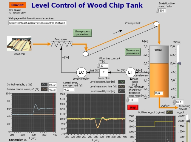
Snapshot of the front panel of the simulator:
Description of the system to be simulated
The level control system for a wood chip tank is simulated. The purpose of the level control is to keep the level between specified limits: It is important that the level is not too high, otherwise the chip will not be sufficiently pre-heated (by steam from the cookery), or the tank will simply run full. And it is important that the level is not too low, otherwise the steam will stream through the chip causing an awful smell in the neighbourhood.
The level control system is (quite) similar to an existing control system at Tofte S—dra Cell in Norway.
The process consists of a chip tank with an inlet screw, a conveyor, and an outlet screw. The inlet flow can be controlled by adjusting the screw control variable. The outlet flow can not be controlled, and it constitutes a disturbance on the level.
Video
Here are a couple of instructional videoe where the present simulator is used as an example:
Mathematical description of chip tank, level sensor and measurement filter
Below is a mathematical model of the process. However, knowledge about this model is not necessary to do the tasks below.
Process model
A mathematical model of the process can be found using a mass balance:
| A*r*dy(t)/dt = Ku*u(t-td) - wout(t) | (Eq. 1) |
- y [m] is the level. y is the process output variable, which is to be controlled.
- u [%] is the control variable, acting on the inlet screw, and giving a proportional mass flow through the screw.
- A [m2] is the cross sectional area of the tank.
- r [kg/m3] is the chip density.
- Ku [(kg/min)/%] is the inlet screw gain.
- td [min] is the transport time of the conveyor belt, which runs with constant speed. td can also be denoted as dead-time or time-delay.
- wout [kg/min] is the mass outflow from the tank. wout is a disturbance on the level.
Dynamically, this process is "an integrator with dead-time" from the screw control.
The values of the model parameters are available via the front panel of the simulator.
Level measurement and measurement filter
The level is measured with a gamma-ray based measurement device having range 0 - 15 m, corresponding to 0 - 100% range. The correspondence between the measurement value ym in percent and the level y in percent is given by the measurement function:
| ym = Km,LT*(y - ym0) | (Eq. 2) |
- Km,LT [%/m] is the measurement gain (LT is Level Transmitter).
- ym0 is the lower limit of the measurement range.
Measurement random noise is added to the level measurement. The measurement signal passes through a lowpass filter which attenuates the noise component of the signal. The filter is characterized by its time constant, Tf [s]. The filter action is removed by setting Tf = 0.
Aims
The aims of the tasks given below are
- to give an understanding of how an automatic feedback control system works, and which benefits feedback control has compared to using a fixed value of the manipulated variable
- to give an understanding of the properties of two important control functions, namely PID control and on/off-control
- to develop skills in tuning controller parameters
- to give insight into how various parameters (in the controller, in the process, and in the measurement device) influates the dynamic properties and the stability properties of the control system.
In other words: This lab will give your (more) insight into the most important issues of control engineering!
Motivation
Control systems are essential in industry because it is important to control process variables so that they are kept equal to or close to set-points. The PID-controller is by far the most frequently used controller function, and it is a main topic in this lab.
This lab is about level control, and in most plants there is a need to control level. The simulated tank with it's level control system in this lab is a "real" system, as it actually exists, as mentioned above.
Suggested exercises
In the tasks below it is assumed that the process is in it's nominal operating point unless something else is stated. The nominal operating point is defined as follows:
- The level reference (setpoint) is 10 m.
- The chip outflow is wout = 1500 kg/min = wout,nom.
- The nominal value of the manipulated variable is unom = 45%, which gives an inflow that is equal to the nominal outflow.
- The filter time constant is Tf = 20 s.
In the tasks about PID-control: Set the set-point weights wp and wd equal to 1, and the coefficient a = Tf/Td equal to 0.1 (these are also the default values as set on the front panel). Let the PID-controller have anti-windup.
- First: No controller! Set the controller in manual mode. Give the outflow a step from e.g. 1500 to 1800 kg/min, which implies that unom no longer fits to the nominal outflow, wut,nom. Characterize the response in the level. Is control using a fixed value of the manipulated variable (unom = constant) an acceptable way of controlling this process?
- Then: Manual control, that is: YOU are the controller! Set the controller in manual mode. Give the outflow a step from e.g. 1500 to 1800 kg/min. Compensate for this disturbance by adjusting unom. How long time do you need to bring the level back to the set-point with an error less than 0.1 meter? Are there any drawbacks with using a human being as a continuous controller?
- Automatic control using
an on/off controller: Set the controller in automatic
mode. Set the on/off controller's amplitude to 10 % and the hysteresis
width to 0%. Give wut and unom
their nominal values.
- Characterize the response in the level. Explain!
- Apply a step to wut from 1500 to 1800 kg/min. How is the response in the level? Explain! What happens with the response if you increase M (from 10%)?
- Automatic control with
a PID-controller: Parameter tuning:
In the tasks above you should have observed that there are certain
problems connected to having a constant manipulated variable, and also
with on/off-control. May be continuous control with PID-controller
will work better?
- Find the PID-parameters using the
éstr½m-Hðgglund-method. (You will see that the response in the
level is not sinusoidal, but just pretend it is - that is, you can
read off the amplitude of the oscillations in the usual way.)
- Find the PID-parameters also using
Ziegler-Nichols' closed-loop method. Are the parameters
approximately the same as with the relay- or on/off-tuner?
In the following tasks you shall use the PID-parameter values as found in task 4a or 4b. If you have not executed task 4, you can use the following PID-parameter values, which you can regard as "standard values":
Kp = 1.8, Ti = 9 min = 540 sec, Td = 2.25 min = 135 sec.
- Find the PID-parameters using the
éstr½m-Hðgglund-method. (You will see that the response in the
level is not sinusoidal, but just pretend it is - that is, you can
read off the amplitude of the oscillations in the usual way.)
- Is the stability of the
control system OK? Give wut a step
from e.g. 1500 to 2000 kg/m, and observer how the level returns to the
set-point. Does the control system have proper stability?
- Compensation properties:
- How large is the stationary control error using a PID-controller after a step in wut from 1500 to 1800 kg/min?
- How long time time does it take for the PID-controller to bring the level back to the set-point with an error smaller than 0,1m (after the step in wut as described above)? Which controller is best in this respect: You, the on/off-controller, or the PID?
- Use a P-controller. Choose a proper value of Kp in the P-controller. How large is now the stationary control error? Zero?
- Tracking properties:
How large is the stationary control error with a PID-ontroller after a
step in the set-point (choose the step value yourself)?
- How the P-, I- and D-term woks:
Observe how the three terms in the control signal, u, works after a step
in the disturbance. (There is a button beneath the diagram of u to show
the time-response of the individual control signal terms.)
- How parameter changes
influences the stability of the control system: Observe
how the stability of the control system changes due to the parameter
changes describes below. In each subtask/experiment you can excite the
control system with a small step in the set-point. The experiments
must be performed independant of each other, that is, you have to
reset the parameters to the standard values (defines above) between each experiment.
- The controller gain Kp is increased (much).
- The integral time Ti is reduced (much).
- The derivate time Td is increased (much).
- The screw gain Ku is increased (much).
- The sampling interval of the controller, Ts_reg (which can be adjusted in the parameter field in the upper part of the front panel) is increased (much).
- The dead-time (time-delay) td of the conveyor is increased (much).
- The cross sectional area A is reduced (much).
- The measurement gain Km,LT is increased (much).
- The set-point gain Km,LC is increased (much).
-
The importance of using the correct measurement function in the setpoint generation:
- What happens with the control error of the set-point gain Km,LC is different from the measurement gain Km,LT?
- What happens with the control error if the lower limit, rm0, of the set-point range is different from the lower limit, ym0, of the measurement range?
-
Measurement lowpass filter: Demonstrate that the measurement lowpass filter attenuates the noise component of the measurement signal. Also demonstrate that the filter reduces the variation of the control signal. (Compare the behaviour of the signals with filter and without filter.) In general, what may be the drawback of large variations of the control signal?
-
Derivative term and measurement noise: Demonstrate that the derivative term of the controller causes the control signal to vary more (compared to not having derivative term).
Updated 12. January 2008. Developed by Finn Haugen. E-mail: finn@techteach.no.