|
|
Introduction to
LabVIEW 8.2
(Ok for 8.5, too)
by
February 12, 2007
This tutorial is freeware!
Contents:
1 Preface
2 Introduction
3 Launching LabVIEW
3.1
License Activation
3.2
Starting using LabVIEW
4 Looking at an
example VI: level_meas.vi
4.1 Downloading and opening the example
4.2
Running the VI
4.3 Studying the
Front panel of the VI
4.4 Studying the
Block diagram of the VI
5 Help
6 Customizing
LabVIEW
7 LabVIEW programming step-by-step
7.1 The aim of the programming:
level_meas_simple.vi
7.2 The programming environment
7.3 General programming guidelines
7.4
Developing the VI
7.4.1
Well-known editing tools apply!
7.4.2
Starting with the Front panel
7.4.3
Then developing the Block diagram
7.4.4
Debugging and testing
7.4.5
VI development continued
8
Additional topics
8.1 Case
structure
8.2 For
loop
8.3
Shift register. Feedback node
8.4 SubVIs
8.5
File writing and reading
8.6 Structuring VIs using parallel While loops
8.7 Text-based programming using the Formula node
8.8 Text-based mathematics using MathScript
8.9
Plotting in graphs
8.10 Generating documentation of your VI
8.11 To
appear...
1 Preface
The aim of this document is to give you an introduction to LabVIEW version 8.2. It is assumed that you have LabVIEW 8.2 installed on your computer. The introduction is to "core" LabVIEW. Thus, no particular LabVIEW toolkit or module is covered.
Only a basic introduction is given, enough to make you able to develop your own LabVEIW programs. If you need additional information, use Help i LabVIEW or search for relevant examples in LabVIEW.
This tutorial is self-instructive, having a number of activities that you are supposed to perform. These activities are shown in blue boxes, as here:
| Activities are shown in blue boxes as this one. |
Please send comments or suggestions regarding this document via e-mail to finn@techteach.no.
More tutorials that may be relevant for you as a LabVIEW user are available from Finn's LabVIEW page.
2 Introduction
LabVIEW is a development system for industrial, experimental, and educational measurement and automation applications based on graphical programming, in contrast to textual programming - however, textual programming is supported in LabVIEW. LabVIEW has a large number of functions for numerical analysis and design and visualization of data.
LabVIEW now has several toolkits and modules which brings the LabVIEW to the same level of functionality as Matlab and Simulink in analysis and design in the areas of control, signal processing, system identification, mathematics, and simulation, and more. In addition, LabVIEW has, of course, inbuilt support for the broad range of measurement and automation hardware produced by National Instruments. Communication with third party hardware is also possible thanks to the availability of a large number of drivers and the support for communication standards as OPC, Modbus, GPIB, etc.
LabVIEW is produced by National Instruments.
3 Launching LabVIEW
You can launch LabVIEW on you PC as follows:
| Start LabVIEW via Start / All Programs / National Instruments / LabVIEW 8.0 / LabVIEW. |
3.1 License Activation
Depending on the way LabVIEW has been installed on your computer, you may be asked by the Activation Wizard to activate the LabVIEW license online (via Web). The activation is done only once on a given PC.
3.2 Starting using LabVIEW
Assuming that the license activation has run without problems, starting LabVIEW opens the Getting Started dialog window shown below.
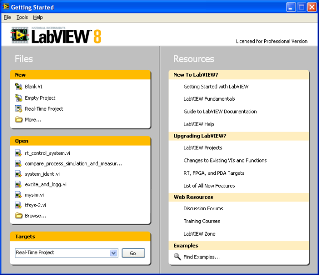
Getting Started dialog window
Here are a comments to the most commonly used options in this dialog window:
- Files / New / Blank VI opens a new, blank VI. VI is short for Virtual Instrument, which represents a program developed in LabVIEW. This is the most commonly used option.
- Files / New / Empty Project opens a new project which is a collection of various LabVIEW files and other files making up a project. (A project is a new construct in LabVIEW 8.)
- Files / Open shows the recently opened files. It is kind of a history list.
- Resources / New to LabVIEW? / Getting Started with LabVIEW links to the Getting Started with LabVIEW PDF document of approximately 80 pages. You may regard it is an alternative to or an addition to the present tutorial. The present tutorial is more directly aimed to developing applications running continuously with a fixed cycle time, as in a control, data acquisition, or a simulation application.
- Resources / LabVIEW Fundamentals links to the LabVIEW Help, where you can find information using the Contents, Keywords, and Search options in the usual way.
- Resources / Find Examples links to the library of examples included in LabVIEW. This library represents a large knowledge base. If you have a specific problem, you will probably find an appropriate example here. The examples are also available via the Help menu in any LabVIEW window.
| Try the items listed above. However, it is assumed that you do not spend too much time on each of them now. (If you open new files, close them without saving.) We will return to several of these items during this tutorial. |
4 Looking at an example VI: level_meas.vi
4.1 Downloading and opening the example
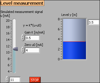
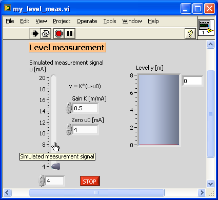
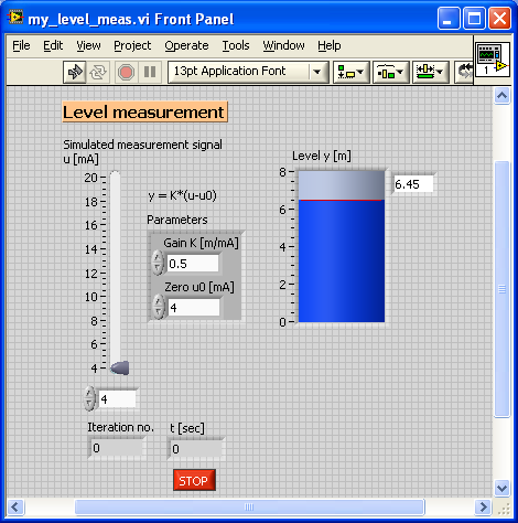
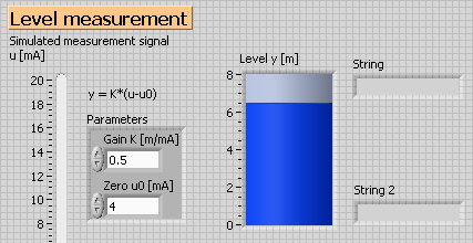
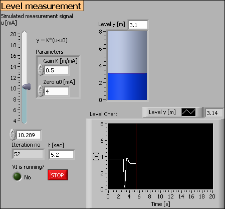
To see how a LabVIEW program works and how it is constructed, let us study the VI (Virtual Instrument) named level_meas.vi which I have made for the purpose of having a simple yet illuminating introductory example. In Sec. 7 of this document you will learn how to develop this VI. This VI converts an assumed (user-adjusted) level measurement signal, u, in milliamperes into a level value, y, in meters according to the following mathematical formula:
y = K*(u-u0)
where K is the gain and u0 is the zero of the measurement. K and u0 can be adjusted by the user. By default, K is 0.5m/mA and u0 is The level value is shown in a tank indicator and in a chart. If the level becomes greater than 7 meters og smaller than 1 meter, a proper alarm is displayed in each case. The program runs periodically with a cycle time of 0.1s. A lamp, or a LED (Light Emitting Diode), indicates if the programs runs or not.
| Download level_meas.vi to any folder (directory) you wish (e.g. C:\temp). Then open the VI via in the Getting Started dialog window. |
Opening level_meas.vi opens two windows:
- The Front panel, which constitutes the user interface of the VI.
- The Block diagram, which contains the program code defining the functionality of the program.
The front panel and the block diagram of level_meas.vi are shown in the following figures. At the moment, disregard the comments added to the figures. We will soon return to the details.
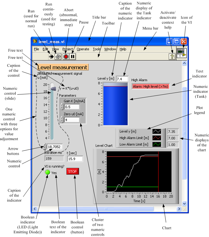
The front panel of level_meas.vi
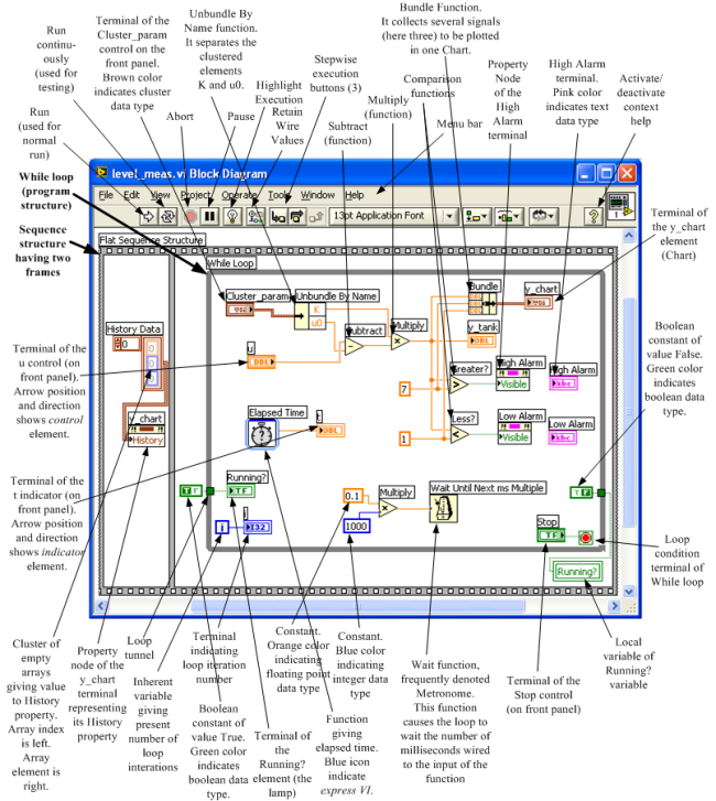
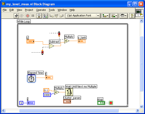
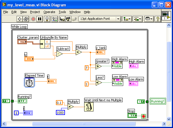
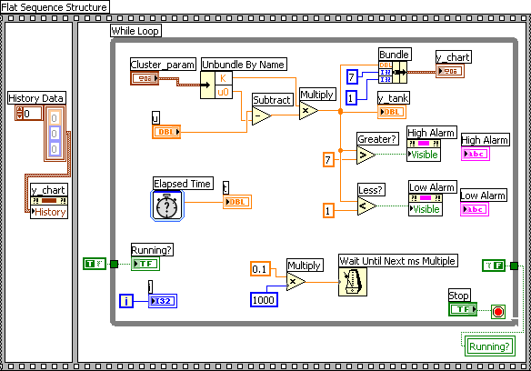
The block diagram of level_meas.vi
4.2 Running the VI
The VI is operated using the buttons on the toolbar, cf. the front panel figure:
- The Run button is used to start the VI. This button becomes white when the VI is not running, and black when it is running. If the VI contains errors, the VI does not start, and the Run button is grey and broken.
- The Run Continuously button is used only for testing purposes when you want to run the VI over and over again. It works as when you continuously click the Run button after the VI has stopped. (Unfortunately many users erroneously clicks the Run Continuously button to run the VI in normal operations. Actually, you need this button very seldom.)
- The Abort button is used to abort the operation of the VI. It is used for abnormal or uncontrolled stop. Typically, the programmer will have put a specific button or switch on the front panel to provide for a controlled stop. In level_meas.vi there is a red stop button at the bottom of the front panel.
- The Pause button is used to pause the VI as it runs. By clicking the Pause button again the VI runs again.
| Run the level_meas.vi. Then play with the VI by
adjusting some of the elements on the front panel. To stop the VI click the
Stop button. Run the VI again. Try the Pause button and the Abort button. |
4.3 Studying the Front panel of the VI
Now that you have played with the level_meas.vi, we will study the contents of the VI in so that you get a more detailed knowledge about LabVIEW. Look at the front panel. It contains two types of elements:
-
Controls. You can adjust the value of a control. A control is an input element.
-
Indicators. These elements are used to indicate values. An indicator is an output element.
State if each of the following elements is a control or an
indicator:
|
Below are detailed comments about the elements on the front panel.
- Description and Tip strip of elements: The programmer may have added a
description and/or a tip strip of a particular element:
Run the level_meas.vi. - To see the Description and Tip strip in a separate window: . Close the display using the OK button in the window that was opened.
- To see the Tip strip: Move the cursor over the vertical pointer slide. The figure below shows the tips strip.
Click the Show Context Help Window button in the front panel toolbar, thereby displaying the description and the tip of the front panel element where the cursor is at the moment. Then, disable the Show Context Help Window button.
- Data types: The front panel elements - both controls and indicators - has a
specific data type. (We will come back to data types in more detail
when we study the block diagram of this VI.) In
this VI there are elements of the following data types:
- Floating point number (decimal numbers)
- Integers
- Boolean or logical elements, which means that the possible values of the element are either On (or True) or Off (or False)
- Text
- Clusters. They contain one or more elements of possibly different data types.
Find at least one front element for each of the data types listed above. (To see a textual element, run the VI and set the value of u greater than 18.)
Answer:- Floating point number: The numerical indicator displaying time.
- Integer: The numerical indicator displaying iteration number.
- Boolean: The Stop button.
- Text: The textual alarm indicator displaying an alarm as the level is greater than 7m.
- Cluster: The element containing the gain K and the zero u0.
- Several options for value adjustment: For one specific control
element there may be several optional ways to adjust the value of the element,
cf. the vertical pointer slide for adjusting u on the front panel. In this example there are three
ways to adjust the value:
- Typing the value
- Clicking the arrow buttons
- Moving the pointer on the slide
Run the level_meas.vi. Try the three different ways of adjusting the measurement value, u. - Several ways to indicate the value: For one specific indicator the
value may be shown in more than one way.
Run the level_meas.vi. Observe that the level is indicated in a chart and in an inherent numeric display. The tank indicator is actually one separate level indicator. - Plots: The present front panel contains one chart plotting
altogether three signals: (1) The level. (2) The High alarm limit, which is 7
(meters). (3) The Low alarm limit, which is 1. In LabVIEW a chart is a continuously updated diagram
with time along the x-axis. You can think of a chart as a pen plotter where
the x axis develops linearly with time. (LabVIEW also has graphs (though
not in this example) which is a more general x-y plot where the x-axis may not show time
but some other values.) The user can change several properties of the chart
even while the VI is running (unless these properties have been programmed to
be non-adjustable):
Run level_meas.vi. - Change the maximum y scale value from 8 to 10 by double-clicking on 8 and editing. Then, reset the value to 8.
- Right-click anywhere on the chart, and select Autoscale Y from the menu that is opened. Then, deselect Autoscale Y, and set the Y axis scaling from 0 to 8.
- Right-click on the plot legend above the diagram to open a menu of plot settings, and change line color, line width, line style, interpolation, point style. Also try some of the bar plots.
- Try the various options available via :
- Hide/show the inherent digital display
- Show/hide X scrollbar
- Show/hide Scale legend
- Show/hide Graph palette
- Try the various options available via :
- Strip Chart
- Scope Chart
- Sweep Chart
- Take a snapshot of the chart via (select the options Emf-file and Save to clipboard in the menu that is opened). Paste the saved image into e.g. a Word document or some photo editor.
- Clear the chart via .
- Free text, captions, and labels: Anywhere on the front panel some
free text may be written by the programmer. For a specific element the
caption of that element may be shown. The caption is a descriptive text
for that element. Furthermore, an element must have a label, which is
the name of the element. When referring to the element as a program variable,
the label is the variable name. The programmer decides wether the caption
and/or the label is shown or not on the Front panel. In the block diagram the
label is always shown. The caption is not shown in the Block diagram.
Run the level_meas.vi. Observe that the tank indicator has a caption (on the Front panel) which is different from the label (the label, not the caption) is always shown on the diagram.
4.4 Studying the Block diagram of the VI
The Front panel is the user interface of the VI. However, the Front panel itself contains no program code. The program code defining the functionality of the program is contained in the Block diagram of the VI.
| It is assumed here that the level_meas.vi does not run. Open the block diagram of the VI using the menu selection . Then use the menu to show the front panel. Also try toggling between the front panel window and the block diagram window using the keyboard shortcut Ctrl E (this is a useful shortcut to remember - it will save you a lot of time during a lifetime with LabVIEW). |
The following are several comments to the block diagram.
The program representation is graphical
A LabVIEW program contains graphical program code, i.e. the code contains various types of elements, blocks and signal wires. (It is however possible to include textual program code in LabVIEW, using e.g. the Formula node or the MathScript node.)
Corresponding elements on the front panel and the block diagram
To any front panel element (e.g. a numeric control or indicator) there is a corresponding terminal in the block diagram. The terminals play the same role as variables in other programming languages, as C, Delphi, Visual Basic etc., and sometimes it is natural to say variable in stead of terminal. Note that terminals look a little different depending on wether it corresponds to a control or an indicator, cf. the examples indicated in the Block diagram. One example is the u terminal in the block diagram. It corresponds to the slider on the Front panel. The value of the terminal and of the front panel element (control or indicator) is always the same. You can find the corresponding front panel element to a given block diagram terminal by double-clicking on the terminal, or by right-clicking the terminal and selecting - or - from the menu that is opened. The reverse operation works, too: You can can find the corresponding block diagram terminal to a given front panel element by double-clicking on the element, or by right-clicking the element and selecting from the menu that is opened.
| Find the Front panel element corresponding to the u terminal. Is the
Front panel element a control or an indicator? Also find the Front panel element corresponding to the y_chart terminal. Is the Front panel element a control or an indicator? |
Data types
Different data types are indicated with different colors. The following data types exist in level_meas.vi:
- Floating point numbers (decimal numbers) are shown in orange color. The letters DBL on the icon is for double, which refers to floating point numbers with double precision, which expresses the numerical accuracy of the internal representation of the number in the computer. You can think of floating point numbers as decimal numbers. One example is the u terminal.
- Integers are shown in blue color. One example is the numeric constant of value 1000.
- Boolean data are shown in green color. The letters TF on the icon is for True/False, which are the two possible boolean (logical) values of the element. One example is the Stop terminal.
- Textual data are shown in pink color. One example is the High Alarm terminal.
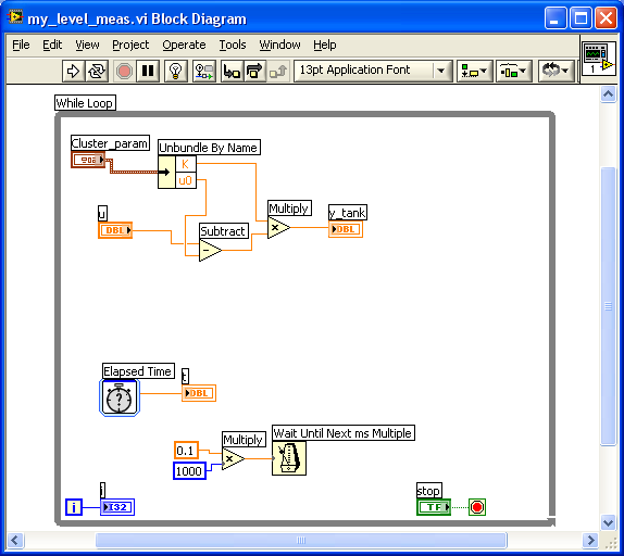
- Cluster data are shown in
brown color. Clusters are multivariables. They contain one or more elements
of possibly different data types. One example is the Cluster_param terminal.
Which two elements are contained in the cluster named Cluster_param?
(Answer: K and u0.)
Constants
Constants are defined values that exist only in the block diagram (so there are no corresponding front panel element). Constants can have various data types, cf. the description of data types above. One example is the constant of value 7 entering the Greater? function.
Locate the following elements on the block diagram:
|
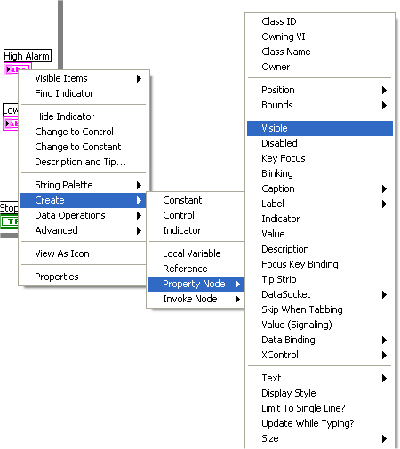
Property node
A property node represents one or more properties of a front panel element. These properties can be either readable or writable. (The latter is typical.) Using property nodes various properties can be set (or retrieved) programatically. Most properties can also be set via the front panel, by right-clicking on the element there.
| Locate the two property nodes to the right in the block diagram of level_meas.vi.
To which elements or terminals do these property nodes belong? Which
property is set (written a value to) in both theses property nodes? What is
the purpose of the property nodes in this case? (Answers: The property nodes belong to the two text indicators named High Alarm and Low Alarm, respectively. The Visible property is set. The purpose of the property nodes is to show them, i.e. to make them visible, on the front panel when the level passes the respective alarm limits.) |
Program execution
A LabVIEW program is executed according to the data flow principle: A block or some other program part is executed only if all inputs to the block has valid values. LabVIEW distributes the execution resources equally to the various parts of the program so that no part is left out.
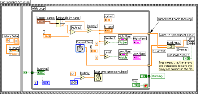
Program structure. Cyclic program execution using the While loop
As seen in the block diagram figure, the progam code is structured using a Flat Sequence structure. The (Flat) Sequence structure is in the form of a film strip with frames. Code can be put into the different frames. The code in the first frame will be executed first, then the code in the second frame, and so on. In the present VI, the code in the first frame writes an empty array to the History property of the chart, thereby emptying the chart just before the cyclic program execution starts. In the second frame is a While loop. The program code inside the While loop frame is executed over and over again cyclically, until the stop condition of the While loop is satisfied. It is the value that is wired into the Loop condition terminal (down left in the While loop) that determines if the loop will stop or continue to run. In this VI the Stop terminal is wired to the loop condition terminal, and hence, this switch is used to stop the while loop. And when the loop stops, any program code outside the While loop waiting for data from some tunnels on the While loop frame will be executed. In this VI the Running? local variable will get value False just after the the While loop has stopped, and after the While loop has stopped the program will stop.
The Metronome function, which is actually denoted the Wait Until Next ms Multiple function, ensures that the cycle time of the While loop is 0.1 seconds. The Metronome actually waits the number of milliseconds wired to the input of the function. In our VI the 0.1 constant is multiplied by 1000 constant to transfer from seconds to milliseconds. Alternatively, we could have wired just a constant of value 100 (ms) into the Metronome.
Note that the Metronome does not implement a time delay of 100ms (in our VI). Suppose, just to take an illustrative example, that LabVIEW uses 2ms to execute the program code inside the While loop (the actual execution time is smaller for our simple program). Then, if the Metronome implemented a time delay of 100ms, the actual cycle time would be 2ms + 100ms = 102ms which is not as specified. In stead, furtunately, the Metronome implements a time delay of 98ms, so that the cycle time becomes 2ms + 98ms = 100ms, as specified at the Metronome input.
Watching and running the execution step-by-step
LabVIEW shows the process of program execution if you click the Highlight Execution button in the toolbar of the block diagram. Furthermore, you can run the program step-by-step by clicking the Start Single Stepping button. These functions are particularly useful for debugging the program since the program execution is shown clearly and in slow speed.
| Run level_meas.vi. Open
the block diagram of the VI. Click the Highlight Execution button in the toolbar, and observe how the program execution is highlighted. Then stop the highlighting execution. Click the Start Single Stepping button in the toolbar to step through the program step-by-step. Stop the single stepping by clicking the Step Out button in the toolbar. |
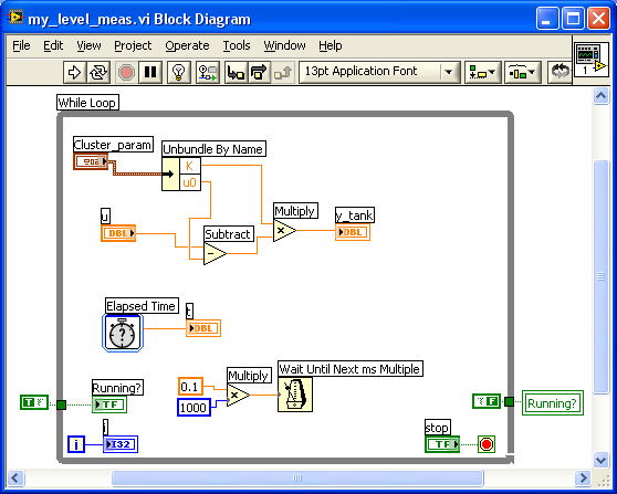
Local variable
A local variable is a copy of a terminal (or variable), and the value of a local variable is the same as the value of the terminal. A local variable can be either writable, or readable. One terminal can have several local variables, being readable and/or writeable. Local variables can be used anywhere within the same VI, but not in another VI - in such cases, you can use shared variables.
| level_meas.vi has one
local variable, namely the local variable corresponding to the terminal
named Running?. Locate this local variable. What is its data type? Try to
explain how the local variable is used in this program. (Answer: Just before the while loop starts, the Running? terminal gets the value of True, thereby lighting the lamp on the front panel. When the user has clicked the Stop button on the front panel, the while loop stops. Just before the while loop stops, the boolean constant of value False is written to the Running? local variable, causing the terminal to get value False, too, thereby turning off the lamp.) |
5 Help
- Help about a specific function in the block diagram: . This opens a Help window for that function.
- Context help: By clicking the Context Help button (with symbol ?) at the right side of the toolbar a context help window is opened. By moving the cursor over an element on the block diagram or on the front panel information about that element is shown in the context help window.
- Help about a topic: Menu: .
Various help (technical documents, application notes etc.) can be found on http://ni.com.
It is assumed that the block diagram of level_meas.vi is opened. Try the various
Help options:
|
6 Customizing LabVIEW
You can customize LabVIEW via the menu. This opens the dialog window shown below. Note that some of the options do not take effect until the next time you start LabVIEW (these options are marked with an asterix, cf. the figure below).
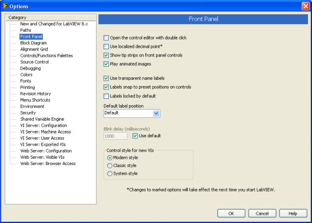
The menu Tools / Options opens the Options dialog window
Below are suggested changes of the default settings:
- Front Panel:
- Disable the Use localized decimal point option. Disabling makes LabVIEW use point as the decimal separator. (If, in stead, this option is enabled, LabVIEW uses the decimal separator as defined in the settings of the Windows operating system.)
- Block diagram:
- Enable Show subVI names when dropped. This causes names of subVIs to be shown in a label on top of the subVI icon (block). A subVI is a LabVIEW subprogram which can be used as a function in the parent program to perform a specific task.
- Disable the Enable auto wiring option. This prevents LabVIEW from automatically connecting adjacent blocks. Although it seems useful to have auto wiring enables, it is my experience that the auto wiring is a little annoying since it tends to draw wires between blocks when you do not want any wire.
- Disable Place front panel elements as icons. This causes LabVIEW
to use small terminal icons on the block diagram. If you, in stead, activate
this option, the terminal icons are larger, with a mimic of the element as it
appears at the front panel. The figure below shows the difference.

The difference between placing front panel elements as icons (i.e. large icon) and not (i.e. small icon)
As seen from the figure, space is saved in the block diagram by not activating Place front panel elements as icons. (I prefer saving space compared to having the more illustrative icons on the block diagram.)
- Alignment Grid: I suggest using alignment grid of 6 pixels on front panel, and no alignment grid on the block diagram.
- Controls/Functions Palettes:
- The Format pull-down list: Category (Icons and Text)
- The Navigation Buttons pull-down list: Label All Icons
- Environment: Disable the Just-In-Time Advice.
| Customize LabVIEW according to the above suggestions or your own preferences. |
7 LabVIEW programming step-by-step
7.1 The aim of the programming: level_meas.vi
We will together create level_meas.vi. Here is the Front panel, and here is the Block diagram of level_meas.vi.
7.2 The programming environment
To start the programming you must open a blank VI:
| Open a new (blank) VI via the menu , thereby opening both a blank Front panel and a blank Block diagram, see the figure below. |
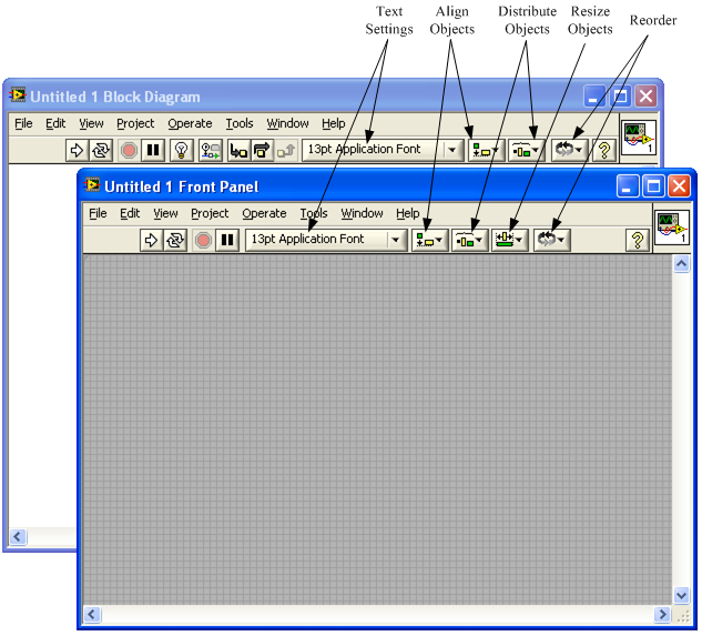
The menu selection File / New VI opens both a blank Front panel and a blank Block diagram
The toolbars of both the Front panel and the Block diagram contain buttons which can be used during the programming, cf. the figure above.
During the programming you will be using the following palettes:
- Tools palette
- Controls palette, which may be opened only when the Front panel is in front of the PC desktop
- Functions palette, which may be opened only when the Block diagram is in front of the PC desktop
These palettes are described below:
Tools Palette
The Tools Palette can be opened by the menu (if it has not already been opened). The figure below shows the Tools Palette.
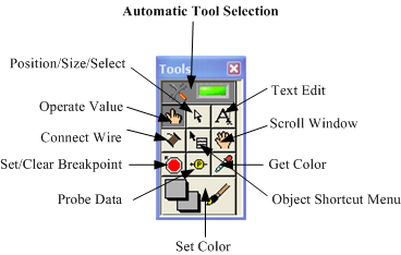
The Tools Palette, which can be opened by the menu View / Tools Palette
| Open the Tools Palette (menu ). |
The Tools Palette contains buttons which you can use to set the cursor in various modes:
- Automatic Tool Selection (default) which lets LabVIEW automatically select the cursor mode, depending on the present position of the cursor. In most cases the automatic tool selection works very fine, hence you do have to care about selecting any of the other buttons in the Tools Palette. (Except when you are going to set colors to elements. Then you will have to select the Set Color button.)
- Operate Value, to changing the value of elements on the front panel or the block diagram
- Position/Size/Select
- Edit Text, to enter text
- Scroll Window
- Object Shortcut Menu, to open a context dependent menu. This button is equivalent to right-clicking on the element.
- Probe Data, to insert probes into the block diagram. A probe is a small vindow showing the value of the wire (line) on which you have clicked. This may be useful in debugging (detecting errors).
- Get Color, to snap the color where you have clicked. This color can then be found in the History list in the color chart window which can be opened using the Set Color button, see below.
- Set Color, to change the color of elements on the front panel or the block diagram.
- Set/Clear Breakpoint, to set and to clear breakpoints in the block diagram. This may be used in a debugging process.
- Connect Wire, to connect elements in the block diagram by drawing wires (lines) between them.
The Controls Palette
The Controls Palette contains sub-palettes which contains the elements that you can put on the front panel. (The Controls Palette actually contains both control elements and indicator elements. Hence, a more accurate, but longer, name would be Controls and Indicators Palette.) The Controls Palette can be opened only when the front panel is in front of the computer desktop. You can open the palette in two ways:
- By the menu
- By right-clicking somewhere on the front panel.
| Open the Controls Palette (menu ). To get a glimpse of the contents, browse the palettes in the two upper rows (these palettes are probably the most frequently used). |
The figure below shows the Controls Palette. Note that new palettes may be added to the Controls Palette due to installation of additional modules or toolkits. Therefore, the Control Palette on your computer may look a somewhat different from the Controls Palette shown in the figure below.
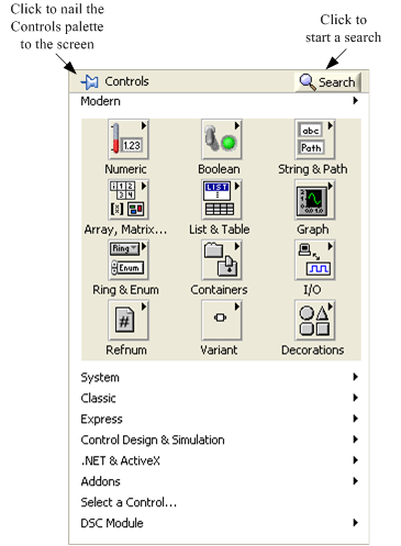
The Controls Palette, which can be opened by the menu View / Controls Palette
The Functions Palette
The Functions Palette contains sub-palettes with functions (blocks) that you can put on the block diagram. The Functions Palette can be opened only when the block diagram is in front of the computer desktop. You can open the palette in two ways:
- By the menu
- By right-clicking somewhere on the Block diagram.
| First, put the Block diagram of your VI in front (e.g. by shortcut Ctrl+E). Then open the Functions Palette. To get a glimpse of the contents, browse the palettes in the three upper rows (these palettes are probably the most frequently used). |
The figure below shows the Functions Palette. Note that new palettes may be added to the Functions Palette due to installation of additional modules or toolkits. Therefore, the Functions Palette on your computer may look somewhat different from the Functions Palette shown in the figure below.
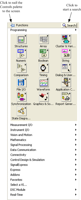
The Functions Palette, which can be opened by the menu View / Functions Palette
7.3 General programming guidelines
Suggested procedure
The programming of a LabVIEW program (a VI) may follow this procedure:
- Elements are placed on the front panel, and then configured by setting various properties (e.g. labels are defined, scales are defined, etc.).
- The functionality of the VI is implemented in the block diagram.
- Additional front panel elements may be added, and additional block diagram code may be added. Note that it is possible to enter front panel elements via the block diagram. This may be quite useful since LabVIEW then automatically creates front panel elements of the correct data type. (This will be demonstrated later.)
Remember to save your work frequently. It may be wise to save the VI under slightly different names as the program evolves, thereby making it easier to retrieve earlier version of the program if the development has taken an adverse direction.
Testing
I have seen many complicated VIs that does not work correctly when they are run the first time, and due to the complexity, it may be very difficult and time consuming to find the errors. In some cases, as if the VI is to control some physical systems, it may be dangerous to run a VI that has not been tested appropriately.
A VI that you develop should not be regarded as complete (finished) until it has been tested! You should test the VI continuously, i.e. at the different stages of the development. The final test should, if possible, be accomplished by some other person than you. (When I work on projects, I always let the user run the VI to give me feedback before I regard the VI finished.)
How do you actually test a VI? It depends on the nature of the VI:
- The VI does not involve communication with any external system
- The VI does involve communication with an external system
These two cases are deescribed below.
The VI does not involve communication with any external system
To test the VI, adjust the front panel elements over all of their ranges of values, including extremal values, so that alarm setting etc. may be triggered. From the observed responses, conclude if the VI, or the part of the VI under concern, works correctly. This testing principle is illustrated in the figure below.
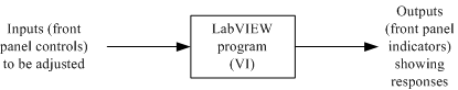
Testing a LabVIEW program can be done by adjusting the inputs over all theirs ranges of values
The VI does involve communication with an external system
Examples are VIs involving I/O (input/output) with physical processes in control applications where the VI calculates control signals as functions of process measurements. When testing the VI you substitute the physical process by a simulated process. The controller function controls the simulated process, and the simulated process feeds measurements back to the controller. This testing principle is illustrated in the figure below. The simulated process can be in the form of a transfer function model or a state-space model representing the differential equations describing the physical process. To learn more about creating simulators and using simulations for testing control systems, see Introduction to LabVIEW Simulation Module 2.0.
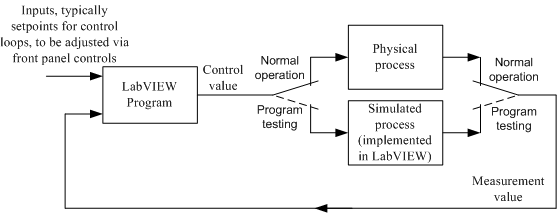
Testing a LabVIEW program for control using simulation
7.4 Developing the VI
7.4.1 Well-known editing tools apply!
The editing tools that you probably are familiar with from text editing etc. also apply in LabVIEW. Here is a list over these tools:
- Undo: Menu , or keyboard shortcut Ctrl+z.
- Redo: Menu , or keyboard shortcut Ctrl+Shift+z.
- Cut: Menu , or keyboard shortcut Ctrl+x.
- Copy: Menu , or keyboard shortcut Ctrl+c.
- Paste: Menu , or keyboard shortcut Ctrl+v.
- Delete: Menu , or Delete key. (Using Delete removes the element without saving it on the clipboard, while Cut removes the element while saving it on the clipboars for a possible later reinsertion.)
- Fine positioning of elements one pixel at a time can be made using the arrow buttons on the keyboard.
Now, let us create level_meas.vi!
7.4.2 Starting with the Front panel
It is assumed that the front panel of a blank VI is in front of the desktop of your PC.
| Save the blank VI with name my_level_meas.vi in any folder you prefer. |
We will now insert elements on the Front panel and configure them according to level_meas.vi.
Free text on the Front panel
Starting with the free text "Level Measurement":
Save the VI. |
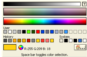
Color palette opened via the Set Color button on the Tools palette
Note: You can set the color of every part of an element on the front panel the same way as you set the color of the text field above, i.e. .
You must also add the free text y = K*(u-u0) to the front panel:
|
Enter the free text "y = K*(u-u0)" on the front panel (with no
particular configuration of the text). Save the VI. |
The Vertical pointer slide
Next, we insert and configure the Vertical pointer slide of the simulated measurement signal, u, cf. level_meas.vi:
|
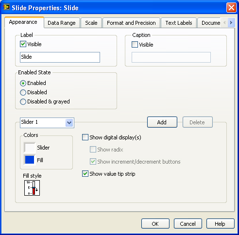
Property window of the Vertical Pointer Slide
About the default value of an element
In the previous activity frame the term default value appear. The default value of an element is the value that the element has just after the VI is loaded into the RAM (random access memory) of the computer, that is, just after you have opened the VI from the permement memory, e.g. the hard disk. Thus, the default value is a start value when the VI is run the first time after being opened. But is the default value also the starting value of en element if you stop the VI and then start it again without closing it? No! In that case the starting value is the value that the element had at the end of the previous run. (So, LabVIEW remembers the latest value.) LabVIEW uses zero as the default default value! If you want some other default value, you can change it via the property window of the element, as you have seen in the activity above. Default values can be set in couple of other ways, too.
Save the VI. |
You can at any time reinitialize the value of an element to its default value:
Save the VI. |
The Gain K element
Next, we insert and configure the Gain K element, cf. level_meas.vi:
|
The Zero u0 element
Next, we insert and configure the Zero u0 element, cf. level_meas.vi:
|
Aligning, distributing, resizing objects
Sometimes you want to align a specific edge of front panel elements to e.g. a common bottom line or to distribute elements with equal space between them or to resize elements so that they get equal size. This can be done using the Align Objects button, the Distribute Objects button, or the Resize Objects button, respectively, on the front panel toolbar.
|
Align the left edges of the Gain K numeric control and the Zero u0 numeric
control: Select both these controls (using the mouse). Then click the Align
Object button on the toolbar and select Left Edges in the palette that is
opened.. Save the VI. |
The Tank indicator
Then, we insert and configure the tank indicator, cf. level_meas_simple.vi:
Save the VI. |
What about the Stop button?
Looking at the Front panel of level_meas_simple.vi, there is still one element on the front panel that we have not put on the Front panel of my_level_meas_simple.vi, namely the Stop button. Although we could very well have placed it on the Front panel as with the other elements, we will in stead place it there via the Block diagram. It is generally useful to be aware of this possibility.
Now, it's time to make the VI work properly! The functionality of the VI is implemented in the Block diagram.
7.4.3 Then developing the Block diagram
The Block diagram so far
The Block diagram of your my_level_meas.vi should be similar to the Block diagram shown in the figure below. So far, the Block diagram just contains the terminals of four Front panel elements. Of course, the Block diagram is completely undeveloped.
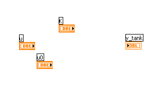
The completely undeveloped Block diagram of my_level_meas.vi after (almost complete) Front panel development
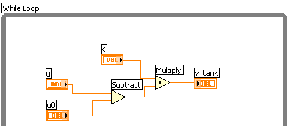
Adding a While loop
Our VI shall run continuously with a cycle time of 0.1s. Therefore, we need to put the code inside a While loop.
|
Insert the While loop: Right-click somewhere up
to the left in the Block diagram (causing the Functions palette to appear) / Select
Structures / Select While Loop, and click to drop it on the Front panel
and with the mouse button still down expand the While loop so that it
embraces the four terminals.
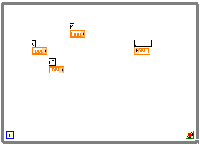
The result should be as in the figure below.
The Block diagram after the While loop has been inserted Save the VI. |
Note: It is essential that code that shall be inside a While loop, programmatically, actually appears (is seen) inside the loop.
Inserting functions
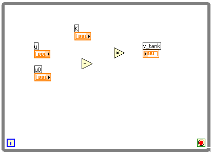
Next, we insert two mathematical functions - the Subtract and Multiply functions into the Block diagram.
The result should be as shown in the figure below.
The Block diagram after the Subtract and the Multply functions have been inserted Save the VI. |
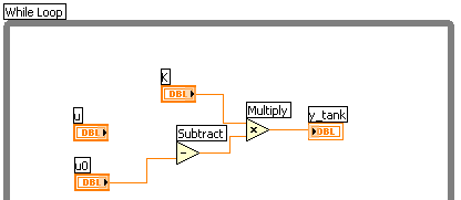
Wiring together elements
Next, we draw wires between the blocks on the Block diagram.
|
Draw the wires in the Block diagram: Move the cursor to a connection point
of either a terminal or a function block, causing the cursor icon to be a
spool. Then (left-)click the mouse, and draw a wire between the elements
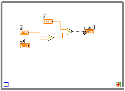
that you want to connect. The result should be as shown in the figure below.
The Block diagram after wires have been drawn using the Connect wire tool Save the VI. |
Wiring tips
Here are a number of useful tips about drawing wires:
- You can draw a wire of any pattern by releasing the mouse button and then moving the cursor before again clicking the mouse and continuing drawing.
- You can delete a wire or a part of a wire in a normal way, i.e. by selecting it with the mouse pointer (single- clicking selects one line segment of the wire, while double-clicking selects the whole wire) and pressing the Delete key.
- If you delete a part of a wire, a broken wire remains. You can delete a broken wire using the Delete key, but you can also use the menu . It turns out that removing broken wires is a frequent operation, and therefore you can save yourself some time by using the shortcut Ctrl + b.
- If you are not happy with the wire route you have drawn, you can let LabVIEW redraw the wire automatically with a resulting "optimal" path: .
Let us try out these tips!
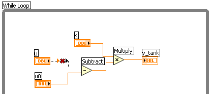
|
Delete the part of the wire between the u terminal and the Subtract function that enters the latter function. The resulting Block diagram is shown in the figure below.
Remove the broken wire going out from the u terminal using the shortcut Ctrl + b. The resulting block diagram is shown in the figure below.
Draw a "crazy" wire from the u terminal to the Subtract function, see the figure below.
Make LabVIEW clean up the long wire between the u terminal and the Subtract function by right-clicking the wire and selecting in the menu that is opened. The resulting block diagram is shown in the figure below.
Save the VI. |
By now, your VI should be similar to level_meas_1.vi. If you want, you may proceed with level_meas_1.vi as the starting point (saving it as my_level_meas.vi in a proper folder).
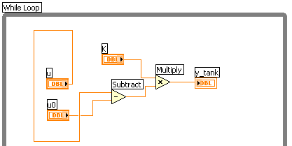
Making labels visible
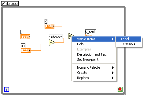
To make your VI even more self-documenting labels of functions and program stucture elements can be made visible.
|
Make the labels of the While loop frame, the Subtract and the
Multiply
functions visible: Right-click on the
element / Visible Items / Label, see the figure below.
The Block diagram after wires have been drawn using the Connect wire tool Save the VI (my_level_meas.vi). |
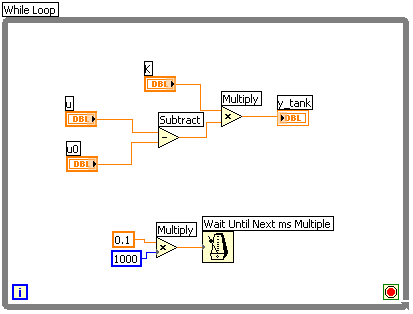
Adding the Metronome (the Wait Until Next ms Multiple function)
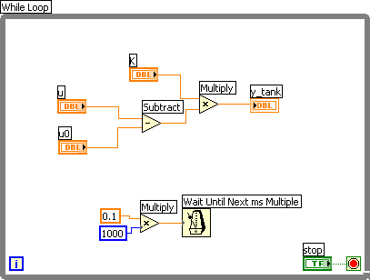
Next, we add the Wait Until Next ms Multiple function, which we for simplicity denote the Metronome function, to implement a cycle time of 0.1s of the While loop. (The Metronome function was explained here.) Since the Metronome must have the cycle time in units of millisensonds at its input, 0.1 is multiplied by 1000, and the product is wired to the Metronome.
The result should be as shown in the figure below.
The Block diagram including the Metronome function (Wait Until Next ms Multiple function) Save the VI. |
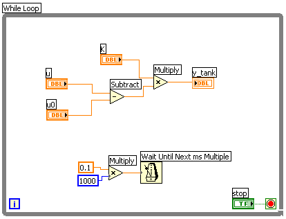
Creating the Stop button via the block diagram
Now we will create a Stop button on the Front panel. As mentioned earlier, we could have put a Stop button on the front panel by selecting from the Controls palette / Boolean subpalette, and then wire its terminal to the Loop condition terminal in the Block diagram. In stead we will create the button from the Block diagram. It is my experience that this is very useful in many cases, since LabVIEW then automatically selects the correct data type (it may be more cumbersome to create manually e.g. a cluster of arrays of numeric element at the Front panel than to let LabVIEW create a correct Front panel element).
|
Create a boolean Front panel element whose terminal will be wired to the
Loop condition terminal:
Right-click on the Loop condition terminal / Create Control. The resulting Block diagram is shown in the figure below.
The Block diagram including the boolean stop terminal wired to the Loop condition terminal |
What was actually created on the Front panel?
| Open the Front panel of the VI (Ctrl+E on the keyboard). |
The figure below shows the Front panel.
The Front panel containing the Stop button automatically created by LabVIEW
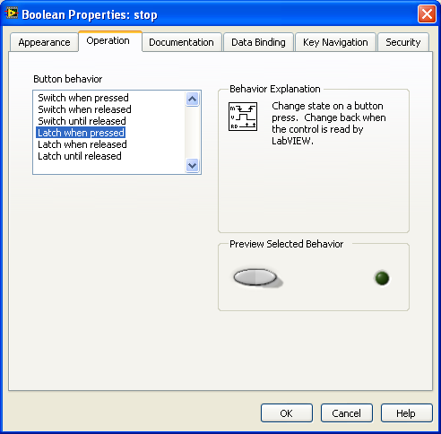
So, the Stop button was placed in the upper left corner of the Front panel. (This is the default position of Front panel elements that are automatically created.) Let us do a few cosmetic changes on the button. Furthermore, we have to make the button operate correctly - a button is not just a button! There are a number of ways a button can operate: It may change its state immediately after having been pressed, or when the press is released. And it may remain in the down-position, or it may pop up as if it is forced by a spring.
|
Move the Stop button to the bottom of the Front panel. Do the following changes to the appearance of the button via its Property window which you open by right-click on the Stop button / Selecting Properties in the menu. The Property window is shown below (with the Operation tab selected, however it is the Appearance tab that is selected by default).
The Operation tab of the Property window of the Stop button
|
7.4.4 Debugging and testing
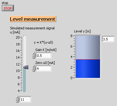
By now your my_level_meas.vi should similar to level_meas_2.vi. The figures below show the Front panel and the Block diagram of level_meas_2.vi. (If you want, you may proceed with level_meas_2.vi as the starting point, starting by saving it as my_level_meas.vi in a proper folder.)
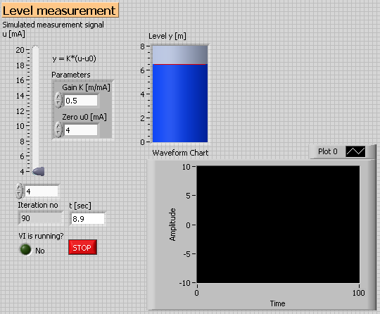
Front panel of level_meas_2.vi
Block diagram of level_meas_2.vi
Hopefully, the VI - my_level_meas.vi - works as assumed. But the only way to confirm it, is by testing it, and of course correcting the errors, which is denoted debugging in computer science.
Detecting and correcting syntax errors (debugging)
Before you can test the VI it must be free of syntax errors, that is, it must have no technical errors. Actually, a VI will not run if it has syntax errors. LabVIEW helps a lot in finding syntax errors. Let us try!
|
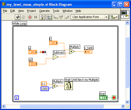
Introduce a syntax error in the VI by deleting a part of the wire between
the u terminal and the Subtract function, see the figure below. Observe that
the Run button is grey and broken!
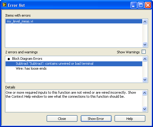
The Run button is grey and broken due to a syntax error Click the Run button to try to run the VI. Since the VI has an error the Error List window is opened, see the figure below.
Error List window Now, double-clicking the first of the two errors in the error list (see figure above), causing LabVIEW to zoom into the error in the block diagram. Fix the error (by completing the wire)! Observe that the Run button now again is normal (i.e. white and not broken). |
Testing the VI to check its functionality
Even though the VI has no syntax errors it may, of course, still not work correctly due to functional errors. It is necessary to test the VI you should operate it through all possible operating ranges and under the various operation conditions while observing the responses and judging if the VI behaves correctly.
With our simple VI we can perform the test as follows:
|
Start (run) and stop the VI a couple of times to check that these operations
work correctly. Run the VI. Adjust the values of u, K and u0 to some integer values (so that it is easy to check the calculations by hand), e.g. u = 10, K = 0.5, and u0 = 4. The VI then produces y = 3. Check this by manual calculations according to the implemented formula y = K*(u-u0). |
With complicated VIs you should test the VI at several stages of its development. (It is like checking that the lower part of the building is safe and strong before you start building the next part upon it.)
While performing functional tests probes, execution highlighting, and stepwise execution may be useful tools to detect errors. These tools are described (and practiced) earlier in this document.
7.4.5 VI development continued
Now that you have got some experience in debugging and testing a VI, we will continue developing the complete level_meas.vi. The following elements will be added to the VI:
- Description and Tip strip of an element
- While loop iteration number (to be displayed in a numeric indicator on the Front panel)
- Clock (for showing elapsed time)
- Cluster (for collecting the K and u0 elements into one cluster element)
- Local variable
- Boolean indicator
- Comparison functions
- String indicators
- Chart (which is a continuously updated plot)
- Property node (for configuration the chart)
Description and Tip strip
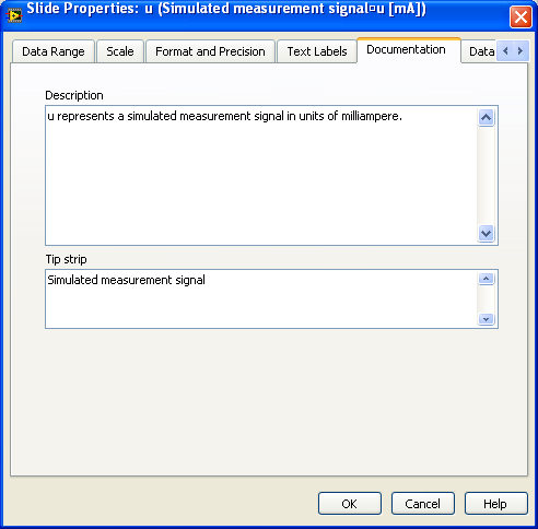
We will add a Description and a Tip strip for the u element (the simulated measurement signal):
|
Open the Property window of the vertical pointer slide of u (right-click on
the element, and select Properties). Open the Documentation tab, and enter
the Description and Tip strip text shown in the figure below.
Description and Tip strip Save the VI. Run the VI and check if the Description and Tip strip are effective:
Tip strip for the vertical pointer slide |
While loop iteration number
To display the Loop iteration number of the While loop, we can connect a numeric indicator to the Loop iteration terminal, see the lower left corner of the block diagram shown in this figure.
|
Open the block diagram of my_level_meas.vi. ,
thereby creating a numeric display indicator at the upper left part of the
front panel. Open the front panel of my_level_meas.vi, and move the indicator to a new position, as shown in this figure. Give the element Label "i" (invisible), and Caption "Iteration no." (visible). Run the VI. Does it seem from the continuously increasing value of the Iteration i element that the While loop runs ten times per second? Stop the VI. Save it. |
Clock
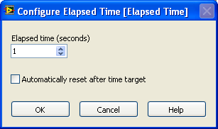
Often we want to have the elapsed time displayed at the front panel. This can be implemented by adding the an Elapsed Time function on the block diagram and displaying the Elapsed Time output of the function in a numeric display on the front panel.
|
Open the block diagram of my_level_meas.vi. Make the While loop somewhat
larger, to make space for the Elapsed Time function to be added, cf.
this figure. Locate the Elapsed Time function on the Timing subpalette on the Functions palette, and add it to the block diagram, cf. this figure. As you drop the block a large blue icon of the function is displayed, and a Configuration window is automatically opened. In this window disable Automatically reset after time target, see the figure below. Then click OK.
Configuration window of the Elapsed Time function Create a numerical indicator to the Elapsed Time output of the Elapsed Time function: . Open the front panel of my_level_meas.vi, and move the Elapsed Time indicator to a new position, as shown in this figure. Give the element Label "t" (invisible), and Caption "t [sec]" (visible). Open the block diagram. The icon of the Elapsed Time function block is large. To use a small icon in stead: . The resulting icon is as shown in this figure. Open the front panel. Run the VI. Does the t element display the elapsed time? Stop the VI. Save it. |
Express VIs
The Elapsed Time function block has a light blue color, indicating it is an Express VI. Express VIs, or Express functions, are actually made of elementary LabVIEW functions. You can configure Express VIs by double-clicking on them. There are many Express VIs on the various subpalettes of the Functions palette.
|
Open the block diagram of a new VI (you do not have to save it, as we will not use it later). Open the following subpalettes, and locate the Express VIs there. You can, to the extent you have time and interesest, drop the Express VIs onto the block diagram to see the configuration window of the Express VI (the configuration window is automatically opened).
|
Cluster
Clusters are elements that contain one or more elements of possibly different data types. We will create a cluster containing the Gain K element and the Zero u0 element. What is the benefits of using clusters? On the Front panel clusters visually groups elements that are somehow related, e.g. controller parameters. On the Block diagram clusters may simplify the code since one cluster wire represents several single wires.
|
Open the front panel of my_level_meas.vi. Add an empty cluster from the
Array, Matrix & Cluster palette to the front panel. The empty cluster may
intermediately be placed anywhere on the Block diagram since we will move it
soon. The figure below shows the Front panel with the empty cluster.
Front panel with empty cluster Now, first drag the Gain K element and then the Zero u0 element into the cluster (you may fine-position the elements using the keyboard arrows). Right-click on the cluster boarder and select . Set the label and caption of the cluster via the Property window of the cluster (to be opened via right-click on the cluster boarder) as follows: Label "Cluster_param" (invisible). Caption: "Parameters" (visible). Move the cluster to the original position of the Gain K and the Zero u0 elements, see the figure below.
The Front panel with the cluster containing the Gain K and the Zero u0 elements Now, open the Block diagram, see the figure below. The Cluster_param terminal has been placed at an more or less arbitrary position.
The Block diagram with the Cluster_param terminal situated (arbitrarily) below the Metronome Next, do as follows. The final result is shown in the figure below.
Block diagram with the cluster terminal and the Unbundle By Name function. Save the VI. |
Boolean indicator. Local variable
We will now add a boolean indicator in the form of a LED (Light Emitting Diode) which will be lightening while the VI runs. Local variables will be used in the implementation.
|
Open the block diagram of my_level_meas.vi. Add a True constant and a False
constant from the Boolean subpalette on the Functions palette, see
the figure below. (Comment: By clicking a
boolean constant the value changes from True to False or from False to
True.) Open the front panel of my_level_meas.vi. Add a LED from the Boolean subpalette on the Controls palette at the position shown here (the LED labeled Running?). Set the properties of the LED as follows (in its Property window):
Note: It may happen that the Caption has a black background color. By double-clicking the Caption field the background color becomes white. Open the block diagram of the VI. Locate the boolean Running? terminal and move it to the position shown in the figure below. Then wire the True constant to the Running? terminal. Create a Local variable belonging to the Running? variable (terminal): . Then, place the Local variable just outside the While loop, and connect it to the False constant, see the figure below. Note: By default a local variable is readable. You can set it to be writable by right-clicking on it and then selecting in the menu that is opened. Block diagram with a True constant connected to the Running? terminal and a False constant connected to the Local variable belonging to the Running? terminal (or variable) Open the Front panel, and run the VI. Observe that the LED is turned on. Stop the VI, and the LED should turn off. Save the VI. |
Comparison functions. String indicators. Property nodes
Now we will implement the alarms. A High Alarm text will be shown on the front panel if the level is greater then 7 meters, and a Low Alarm text will be shown if the level is less than 1 meter.
We start by adding String indicators which will be used to display the
alarms.
Now we will add the necessary functionality to the block diagram. While following the instructions below, refer to the figure just below showing the resulting block diagram. Block diagram with Comparison functions, text indicators and property nodes
Open the front panel, and run the VI. Adjust the value of u to the maximum value and then to the minimum value. Are the alarms displayed correctly? Save the VI. |
Chart
We will now add a chart to our VI. A chart is a continuously updated diagram for plotting variables with time along the x-axis. In our VI the chart will plot three signals:
- The level.
- The High alarm limit, which is 7 (meters)
- The Low alarm limit, which is 1
Adding a chart
|
Open the front panel of my_level_meas.vi. Add a chart at the position shown in the figure below. The chart is found at .
A (waveform) chart is added to the Front panel |
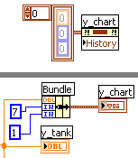
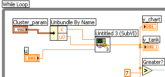
The (three) signals to be plotted in the chart are collected using a Bundle function in the Block diagram. The Bundle function produces a cluster of signals, and this cluster is then wired to the chart. The relevant resulting part of the Block diagram is shown in the figure below.
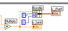
Using a Bundle function to collect the signals to be plottet in the chart
|
Now, let us do some changes to the chart on the Front panel:
|
There is a large number of options when configuring a chart. We will now add a chart with typical basic settings. We will mostly make the settings in the Property window of the chart. Later you will see how to configure the chart programmatically, i.e. by wiring values (constants) to a Property node of the chart in the Block diagram.
Basic settings via the Property window of the chart
|
To configure the chart, open its Property window (by right-clicking somewhere on the chart). Then do the following setting in the different tabs:
To set the Plot legend (above the diagram, to the right) properly:
Open the front panel. Run the VI, and play with the u value. The y-axis has automatic scaling, which is the default setting. Change to manual scaling while the VI runs by right-clicking on the chart, and selecting AutoScale Y. |
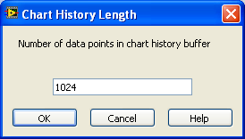
The chart has an inbuilt data buffer which stores previous (historical) data so that the previous signal values are shown in the chart. The default length of this buffer is 1024. Thus, at each instant of time the most 1024 recent samples of the signal are stored in this buffer. In our VI, with a sampling time of 0.1s and a range of 50s along the x-axis, the buffer must have a length of 50s/0.1s = 500 samples. Therefore the default buffer length is ok in our case. But in other cases it may be necessary to increase the buffer length.
|
To see/set the buffer length: Right-click on the chart / Select Chart History Length, see the figure below. However, as argued above, it is not necessary for us to change the buffer length, so you can just close the dialog window.
The Chart History Length can be seen/set via Right-click on the chart / Chart History Length |
Programmatic configuration of the chart
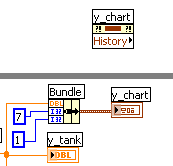
As an example of programmatic configuration of the chart, we will set the History property of the Property node of the chart in the Block diagram so that the chart is emptied as the VI starts.
|
Open the block diagram of my_level_meas.vi. Do as follows:
Next, we have to ensure that the added code is executed before the While loop starts. This can be done using a Sequence structure which is in the form of a film strip with frames. Code can be put into the different frames. The code in the first frame will be executed first, then the code in the second frame, and so on. Add a Flat Sequence from the Structures palette (on the Functions palette), and ensure it embraces the While loop, see the figure below.
A Flat Sequence structure embracing the While loop Then, do as follows:
The resulting block diagram is shown in the figure below.
Block diagram with a Flat Sequence structure Open the Front panel, and Run the VI. Adjust the input signal u. Stop the VI, and run it again. Is the chart emptied at the moment the VI is started, as expected? |

8 Additional topics
8.1 Case structure
A Case structure consists of a number of different cases or frames containing their individual LabVIEW code. Only one of the cases is active at any instant of time. The Case selector selects or controls which one among the cases is active. So, a Case structure implements a way of selecting among alternative portions of program code. The Case structure in LabVIEW si similar to the case or switch structure in other programming languages
case.vi is a simple example of a Case structure. The Case structure is used to display alternative texts in the String indicator, depending on wheter the value of u adjusted with the vertical slider is greater than (or equal to zero) or less than zero. The figures below show the Front panel and the Block diagram of this VI.
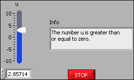
The Front panel of case.vi
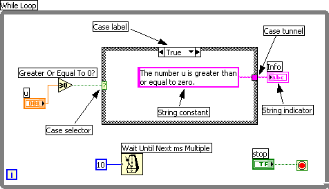
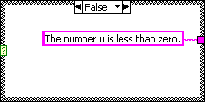
The Block diagram of case.vi. The two alternative cases (frames) are shown. The True case is shown in the upper part of the figure, and the False case is shown in the lower part.
Comments to case.vi:
- The comparison function named Greater Or Equal To 0? is used to generate a proper Boolean value - True or False - which is wired to the Case selector.
- The two Cases are identified by the labels True or False, respectively.
- String constants contains the alternative strings to be displayed in the String indicator on the Front panel.
- Values out from (or into) Case frames are transferred via tunnels. Tunnels are automatically created if as you draw a wire across a Case frame. All output tunnels, i.e. tunnels for signals leaving frames, must be wired to some signal. This is the case in the Block diagram shown above. A String constant is wired to the output tunnel of each of the two frames. (Honestly, you may drop wiring a value to an output tunnel, but if so, you have to tell LabVIEW to use the default value of the indicator to which the tunnel is wired in stead. This is done via right-click on the tunnel.)
You may want to try adding a Case structure yourself:
|
Finally, some general comments to the Case structure:
- In our example, case.vi, the Case structure Labels have Boolean values, True and False, and the Selector must then recieve a Boolean value, too. However, you may use other data types for the Labels and the Selector, for example an integer type or an enumerate type, making it possible to select among any number of alternative cases. Once you wire say an integer signal to the Selector, the Label is automatically adopted to that data type, getting Labels 0, 1, 2.
- You can edit the Case structure (e.g. removing cases, adding cases, swapping cases, defining a given case to be Default, which means that this case is active if the there is no Label match the present Selector value.
8.2 For loop
The For loop is a program structure which can be used to run a certian amount of program code over and over again a predefined number of times. The For loop is quite similar to the While loop, however, as said, with the For loop the number of loop iterations is fixed (predefined) while with the While loop that number is not predefined.
Let us look at an example of a For loop. The program reads successively new values from an array according to the following pseudo code:
Arr1 = [10,20,30,40,50,60,70,80,90,100];
N = 5;
for
i = 0:N-1
{
x = Arr(i);
}
The VI for_loop.vi implements this code in LabVIEW. The Front panel and the Block diagram of this VI are shown in the figures below.
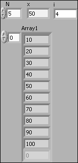
The Front panel of for_loop.vi
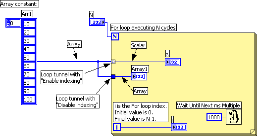
The Block diagram of for_loop.vi
Comments to for_loop.vi:
- The N terminal of the For loop defines the number of execution cycle times. N is set to 5 on the Front panel.
- For demonstration purposes I have placed a Metronome (the Wait Until Next ms Multiple function) with Wait time of 1000ms = 1s inside the For loop to make it possible for the user to follow the changes of the values on the Front panel as the VI runs.
- I have put yellow colour to the For loop just to highlight the loop.
- The i terminal is the For loop index. Its value increases by one, starting from zero, each time the For loop executes. The i terminal is available for you to use in your code.
- Arr1 is an array constant which I have manually fed with values.
- The array enters the For loop via two Loop tunnels which are set up in
different ways, just to demonstrate important features of For loops:
- Via a Loop tunnel with setting Enable indexing. In this case, what comes out from the tunnel is the value (a scalar) of the array element having the same index number as the present value of the For loop index. Thus, in our VI the For loop automatically reads successive array elements as the For loop executes and displays the element in the x indicator on the Front panel. Since the
- Via a Loop tunnel with setting Disable indexing. In this case, what comes out from the tunnel is the entire array. In our VI the entire array is displayed in the Array1 indicator on the Front panel.
You may want to try adding a For loop to a VI yourself:
|
8.3 Shift register. Feedback node
In LabVIEW a Shift register is a memory element storing values from previous executions of loops, e.g. While loops and For loops. A Shift register can store values of any type, e.g. integers, decimal number (floating point numbers), arrays, clusters. A Feedback node is (almost) equivalent to a Shift register. It has less features than a Shift register, but appears somewhat different in the Block diagram. Both Shift register and Feedback node will be described in the following.
Shift register
Let us look at a simple example where a Shift register is used to implement the recursive formula
y(i)=y(i-1)+u(i), with initial value y(-1)=2
where i is the time index (which counts the discrete time steps), which starts on zero. The figures below show the Front panel and the Block diagram of shiftregister.vi.
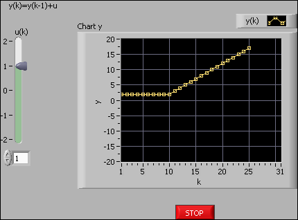
Front panel of shiftregister.vi
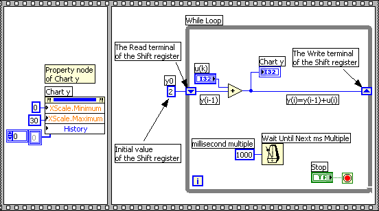
Block diagram of shiftregister.vi
The user can adjust the control u (an integer) while the VI is running. A Shift register is used to store y(i) so that it becomes available as y(i-1) in the subsequent execution (or cycle) of the While loop, and y(i-1) is used in the calculation of y(i), cf. the formula given above.
You may want to try create a Shift register yourself (by first removing the existing Shift register and then immediately creating a new one):
|
The Shift register in shiftregister.vi stores a value created in the previous cycle of the While loop. What if you want to store older values than just the previous value? No problem - just expand the left Shift register terminal by dragging the bottom line of the terminal downwards. And you can assign initial values to each of the elements of the Shift register, see the figure below.
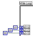
The Shift register may contain values from older cycles of the While loop
Feedback node
The figure below shows a Feedback node. It can store the value of an element from one previous loop cycle (whereas a Shift register may store values from even older cycles). A Feedback node appears somewhat simpler in the block diagram.
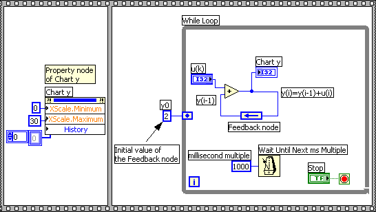
A Feedback node, which is (almost) equivalent to a Shift register
You can create a Feedback node in two ways:
- By replacing an existing Shift register with a Feedback node
- By inserting a Feedback Node from scratch
Let us try both ways.
Creating a Feedback node by replacing an existing Shift register:
|
Creating a Feedback node from scratch:
|
8.4 SubVIs
What is a SubVI?
In all programming languages, e.g. Visual Basic, C++, Delphi, MATLAB, you can create your own functions which can be used in - or be called by - the main program. Similarly, in LabVIEW you can create your own SubVIs. A SubVI is a special kind of VI as it has input and/or output connectors. SubVIs are used in the same way as function blocks in the Block diagram and they communicate with the rest of the Block diagram via the connectors on the SubVI block.
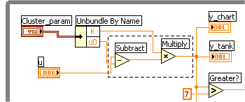
The figure below shows an example of a Block diagram containing the SubVI named sub_vi.vi. The Block diagram belongs to a VI similar to level_meas.vi. The SubVI implements the mathematical formula
y = K*(u-u0)
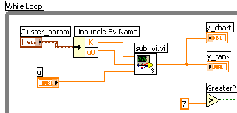
Block diagram containing the SubVI named sub_vi.vi
A SubVI has a Front panel and a Block diagram. By double-clicking on the SubVI block, the Front panel is opened, and then the Block diagram can be opened in the usual way. As you see in the figure below, the Block diagram implements the formula y = K*(u-u0).
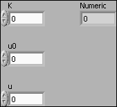
Front panel of the SubVI sub_vi.vi
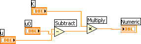
Block diagram of the SubVI sub_vi.vi
The Front panel controls (and their corresponding Block diagram terminals) represent input connectors on the SubVI. The Front panel indicators (and their corresponding Block diagram terminals) represent output connectors on the SubVI.
Where are the connectors of the SubVI? You can see them by right-clicking the SubVI icon which is the icon at the upper right corner of the Front panel window, and selecting in the context menu, see the figure below. By clicking one of the connectors in the Connector pane, the corresponding element on the Front panel is highlighted. In the figure below the connector corresponding to the K element is selekcted and the K control element is thereby highlighted.
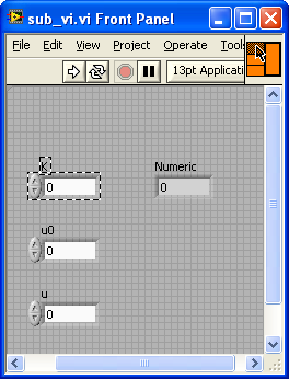
The Connector pane of the SubVI sub_vi.vi
Why would you use a SubVI? You can use a copy of the SubVI in several places in one or more Block diagrams, thereby reusing code effectively. For example, you may implement a mathematical formula in a SubVI. Furthermore, you can also make your Block diagram look simpler by putting code into a SubVI.
How to add an existing SubVI to the Block diagram
As an example, let us add an existing SubVI to the Block diagram of an existing VI. (The application is based on level_meas.vi.)
|
How to create a SubVI
In the above section we added an existing SubVI into a Block diagram. But how do you create a SubVI? It can be done in two ways:
- Manually: You start with a blank VI and develop it further as a SubVI.
- Automatically: You start with some existing Block diagram code that you want to put into a SubVI, and tell LabVIEW to create a SubVI based on that code.
In the following only the automatic method will be described in detail.
Let us try to create a SubVI using the automatic method:
Block diagram containing the SubVI named sub_vi.vi |
Here are a few additional comments to SubVIs:
- File saving:
- The ordinary menu just saves the main VI.
- To save also the SubVI(s), select the menu .
- To save all the involved files (here: the main VI and the SubVIs) into one LabVIEW Project file (however, LabVIEW project is not described here): , thereby opening a Save As dialog window. In this dialog window, select the Duplicate hierarchy to new location option, etc.
- Editing the SubVI icon: Open the Icon
Editor as follows: Right-click the SubVI icon which is the icon at the upper
right corner of the Front panel window, and then select
in the context menu, see the figure
below. Now you can edit the icon using the graphical tools at the left part of
the editor.
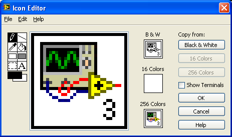
The Icon Editor
-
Setting a SubVI to become reentrant: If several copies of the same SubVI will be used in one, or in several Block diagrams (of other VIs) it is important that each of these copies are independent of each other. This is implemented by making the original SubVI reentrant. To define a SubVI as reentrant: Right-click on the SubVI icon in the upper right corner of the SubVI Front panel / Select VI Properties / Select Category: Execution / Select Reentrant Execution.
-
Editing the SubVI: You can edit a SubVI as you would edit any VI, e.g. you can add code to the Block diagram. You can also add or remove Front panel controls and indicators corresponding to new SubVI inputs or outputs, respectively. To edit the connectors (representing the SubVI inputs and outputs): Right-click on the SubVI icon in the upper right corner of the SubVI Front panel / Select Show Connector, therby opening a context menu containing several options for editing the Connector pane, cf. this figure. For example, you can add and remove inputs/outputs, can change the pattern of the connectors, disconnect a connector from a Front panel element, etc.
8.5 File writing and reading
Introduction
Some times you want to save data generated while a VI was running permamently in a file, and sometimes you want to read data into a VI from a file. LabVIEW has a large number of functions for such File I/O (Input/Output) on the File I/O subpalette on the Functions palette. There are functions for continuous file write and read and for batch (or discontinuous) file write and read.
If your application requires writing historical data (i.e. data generated over a time interval) to a file, you should consider using a file writing function that writes the data in a batch, typically after the VI has stopped, in stead of using a continuous file writing function. The latter may slow down the cycle time of the VI because it takes time for the PC to accomplish this continuous mechanical operation of the PC hard disk. Data to be written in a batch can be intermediately stored in arrays in your VI, and then the array is written to file. This is shown in the example described below.
File formats
The most important file formats in LabVIEW are datalog and text:
- Datalog files are binary files in an internal LabVIEW file format. Datalog files may contain data of any LabVIEW data type, as integer, floating point numbers, Boolean data, clusters. The datalog format gives great fleksibility and effective data storage. Datalog files may however not be opened in other programming tools than LabVIEW.
- Text files or ASCII files or Spreadsheet file are files that contains data that can be read by a human being. Numbers are represented as text. For example, the number 0.231 is stored as the text (or string) "0.0231". A large benfit of storing numerical data in the text format is that the file can be opened and displayed in any tool that supports text files, e.g. MS Word, Notepad, Excel, Matlab, Web browsers. Thus, text files provides great portability. However, the text file format is not optimal, i.e. the file may become larger than a corresponding Datalog file.
As a general rule I suggest that you use the text file format sue to its great portability.
Writing data to a text file
Let us go directly to an example: The figures below show the Front panel and the Block diagram of spreadsheet_file_write.vi. (This file is based on level_meas.vi.)
Front panel of spreadsheet_file_write.vi
Block diagram of spreadsheet_file_write.vi
Comments to the block diagram of spreadsheet_file_write.vi:
- The Write To Spreadsheet File function writes the file. The input labeled file path is not wired in the Block diagram of our VI. Since this input is not wired a file path dialog window is opened just before the file writing begins, and you are asked to give a file name. When I ran this example, I used file name data1.txt in a proper folder.
- The output tunnels of the While loop contains the arrays that are written to the file. These tunnels have been set to Enable Indexing (this is set via right-click on the tunnel).
- The two 1 dimensional arrays are collected into a 2-dimensional array in the Build Array function. Note: It is crucial that the 1-D arrays are not concatenated. This is set by right-clicking on the Build Array function and deselecting in the context menu.
- The 2-D array out from the Build Array function is wired to the 2D (two dimensional) input on the Write To Spreadsheet File function (there is a 1D input, too).
- The transpose? (no:F) input to the Write To Spreadsheet File function is set to True (thus transposing is taking place) to make the arrays appear as columns in the resulting text file. (Columns format is more convenient than rows format in most cases.)
The result of running spreadsheet_file_write.vi is a text file named data1.txt. The figure below shows part of this file opened the Notepad text editor.
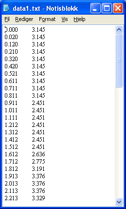
Part of the data1.txt file opened in Notepad
Reading data from a text file
Let us look at an example: The figures below show the Front panel and the Block diagram of spreadsheet_file_read.vi.
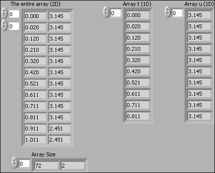
Front panel of spreadsheet_file_read.vi
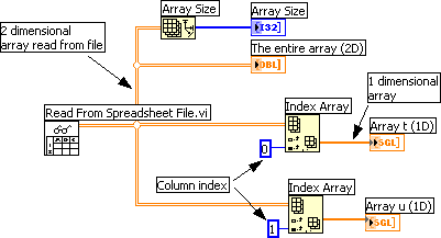
Block diagram of spreadsheet_file_read.vi
Comments to spreadsheet_file_read.vi:
- The Read From Spreadsheet File.vi function reads data from a text file. If you run this VI you will be prompted which file to open. (If I had wired a Path constant or Path control terminal to the File Path input to this function, the file reading would take place automatically without any file name prompt.)
- The output from the Read From Spreadsheet File.vi function is a 2 dimensional array containing the two columns of data, cf. the Data1.txt file.
- The two Index Array functions are used to extract each of the columns from the data and create 1 dimensional arrays, labeled Array t (1D) and Array u (1D) in the example.
- The Block diagram also contains code for displaying the array in an array indicator and to display the size of the array on the Front panel.
8.6 Structuring VIs using parallel While loops
Often your application implements a number of different tasks to be executed simultaneously, e.g.
- Reading measurement signals from input devices
- Signal processing, e.f. lowpass filtering
- Simulation
- Calculation of a control signal using a feedback controller, e.g. a PID controller
- Writing control signals to output devices
- Plotting data in charts on the Front panel
- Saving data to a file
One conventient way to organize such parallel tasks is to put the tasks into individual While loops that run in parallel (simulateneously). These While loops may run with different cycle times. LabVIEW will allocate resources to each While loop (parallel tasks) so that each get a cycle time equal to or close to the cycle time set by the Metronome function (Wait Until Next ms Multiple).
Here is an example: Below are the Front panel and the Block diagram of parallel.vi.
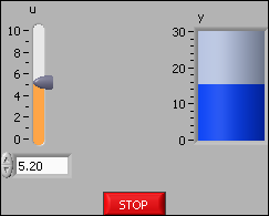
The Front panel of parallel.vi
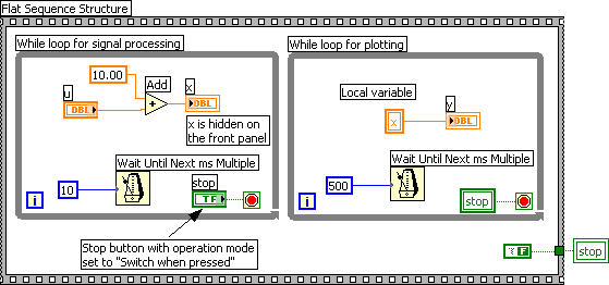
The Block diagram of parallel.vi
Comments to parallel.vi:
-
The VI adds 10 to a user adjusted value of u (this is denoted Signal processing in the Block diagram). The resulting value is then plotted in a Chart (denoted Plotting).
-
The VI contains two parallel While loops inside a Sequence structure. The two While loops implements signal processing and plotting, respectively.
-
The While loops runs with different cycle times, 10 and 500 ms, respectively.
-
Data is transferred from the Signal processing loop to the Plotting lopp using a local variable of x.
-
The x indicator is hidden on the Front panel (Right-click on the element / Hide indicator).
-
One Stop button is used to stop both loops. A Local variable of the button is used to stop the Plotting loop. Note: It is necessary that the button remains in the down position until both loops have stopped. Therefore the mechanical operation mode of the button is set to Switch when pressed. This is set in the Properties window of the Stop button, see the figure below.
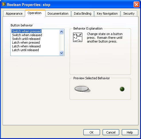
The button behaviour is set to Switch when pressed in the Property window of the button
When both loops have stopped, the Stop button must of cousre pup out again. This is implemented with the Sequence structure embracing both While loops, and with the False constant being written to a Local variable of the Stop button outside the Sequence structure.
8.7 Text-based programming using the Formula node
The Formula node is a window in the block diagram where you can write textual program code following the C-syntax. Using a Formula node for mathematical expressions is often more convenient than building the expression using elementary blocks in the ordinary graphical way in LabVIEW since it is easier to write and maintain textual mathematical expressions than drawing equivalent block diagram code.
Here is the interesting part of the block diagram of the VI formula_node.vi where the Subtract and Multiply functions have been replaced by a Formula node containing the textual code
z = u-u0;
y = K*z;
The VI is otherwise the same as level_meas.vi.
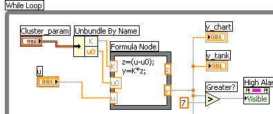
Block diagram of the VI formula_node.vi where the Subtract and Multiply functions has been replaced by a Formula node containing the textual code
|
Add a Formula node to the block diagram as follows:
|
You may wonder why you entered the code
z = u-u0;
y = K*z;
in stead of the somewhat simpler
y = K*(u-u0);
Actually, the latter would work perfect. However, often you will want to split an expression into smaller parts each consisting of expressions (which must be ended with a semicolon), and then having one final expression based on the intermediate results from these expressions. In such cases, remember to define one output for each of the left-hand variables used in the expressions. What actually happens is that each variable is defined. It is not necessary to wire the outputs to some terminal of functions outside the Formula node. As an alternative to defining variables using such "dummy" outputs, you can use ordinary variable declaring expressions as in the C language. In our case we could have used the following code:
float z;
z = u-u0;
y = K*z;
8.8 Text-based mathematics using MathScript
MathScript is a LabVIEW tool for executing textual mathematical commands (or expressions). Please see the Introduction to MathScript.
8.9 Plotting in graphs
You have already learnt to plot signals in Charts. A Chart is continuously updated by the most recent signal values, and the x axis is typically the time axis. A graph is another type of plots. Graphs plots any array versus any other array in an XY (and the increment in the X array does not have to be constant). There are several Graphs on the Graph palette on the Functions palette, the most general being the XY Graph.
Here is an example based on a somewhat simplified verson of level_meas. The three arrays consisting of the historical values of the y, y_max, and y_min are plotted against one time array containing the discrete times covering the elapsed time as the VI was run. The Chart is updated once the While loop has stopped. (The VI also contains a Chart, which is continuously updated as the VI runs.) Below are the Front panel and the Block diagram of graph.vi.
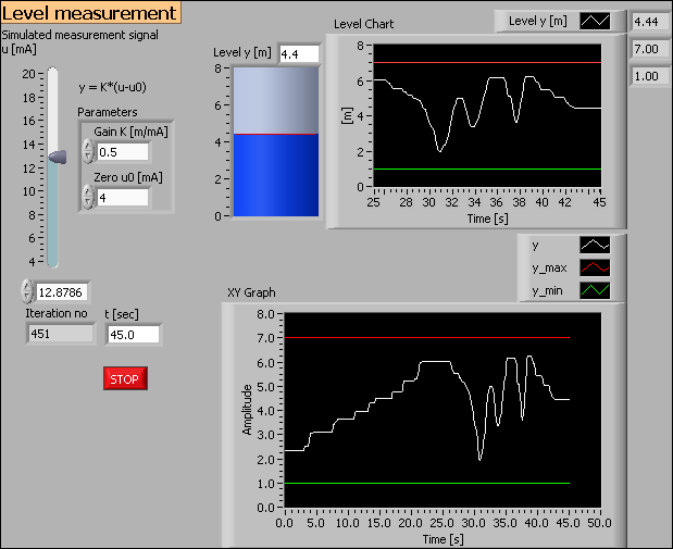
Front panel of graph.vi
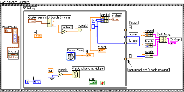
Block diagram of graph.vi
Comments to this VI:
- The XY Chart indicator is available on the Controls palette / Graph subpalette.
- In the Block diagram of graph.vi the XY Graph terminal is placed outside the While loop. This is necessary since the Chart is to be updated once the While loop has stopped. (The Chart terminal is however placed inside the While loop since it is to be updates as the While loop runs.)
- The arrays of y, y_max, y_min, and t are generated in the respective tunnels on the right border of the While loop. These tunnels are set to "Enable Indexing" (this is set by right-clicking on the tunnel and selecting Enable Indexing in the context menu).
- Bundle functions are used to bundle the t array with the y array, the t array with the y_max array, and the t array with the y_min array. The output of a Bundle function is a cluster. Then, these three clusters are collected using a Build Array function. The resulting array of clusters of arrays (!) is then wired to the XY Graph terminal.
8.10 Generating documentation of your VI
You can create a documentation of your VI with various outputs:
- Paper print
- An HTML file which may be shown in any Web browser. Graphics show the Front panel and the Block diagram of the VI. You can edit the resulting HTML file in any HTML browser, e.g. Microsoft's FrontPage. The graphics files are ordinary graphic files.
- A RTF document which can be opened in various editing tools, e.g. Microsoft Word and Scientific Word.
- A plain text document containing no graphics.
The figure below shows one such HTML file opened in a Web browser (Opera).
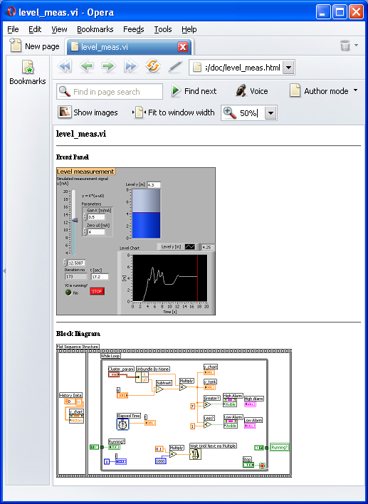
A documentation HTML file opened in a Web browser (Opera)
Creating the documentation is done via the menu. This opens a number of successive dialog windows which are not described in detail here. However, one tip for generating an HTML file is to select True color in the dialog window shown below, otherwise some colors on the Front panel may look strange in the resulting document.
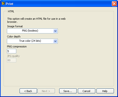
The dialog window where you select Color depth. There you should select True color.
Let us try:
|
8.11 To appear...
- Shared variables...
- LabVIEW projects...