Transfer Function

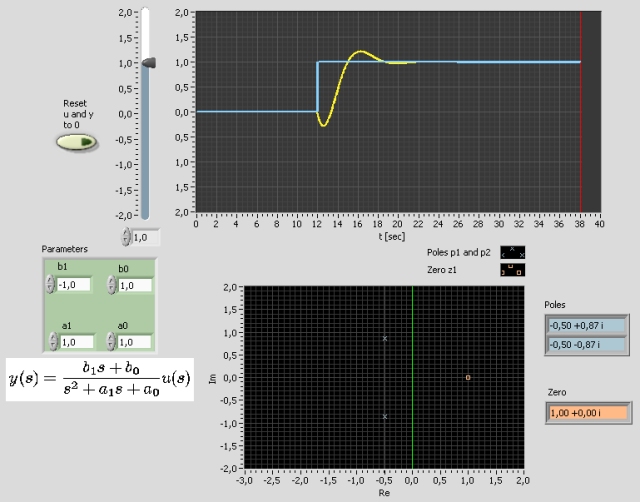
Snapshot of the front panel of the simulator:

• What is needed to run the the simulator? Read to get most recent information!
• Tips for using the simulator.
• The simulator: transferfunction.zip (unzip, and open transferfunction.exe).

Description of the simulated system

The following general second order transfer function model is simulated:

y(s)/u(s) = H(s) = (b₁s + b₀)/(s² +  a₁s + a₀)

H(s) can have both poles and zeros. You can determine the coefficients of the numerator and the denominator polynomial.

Aims

The aims of this simulator is to develop the understanding of the relation between poles and zeros and the time response of transfer function models.

Motivation

Transfer function models are frequently used in signal processing (to represent signal filters) and control  theory (to represent process models, controllers, and sensors).

Tasks

It is assumed that you answer the following questions by running the simulator.

1. Is it confirmed that the system is unstable if the system has at least one pole in the right half plane? (You may set b₁ = 0; b₀ = 1; a₁ = -0.2; a₀ = 1;)
2. Is it confirmed that the system is on the stability limit if the system have poles on the imaginary axis (and no poles in the right half plane)? (You may set b₁ = 0; b₀ = 1; a₁ = 0; a₀ = 1;)
3. Find (by calculation) the static transfer function H_s of the system. Assume that the input u is a step of amplitude U. Calculate the corresponding static response, y_s. Is the resultat confirmed in a simulation? (You may set b₁ = 0; b₀ = 1; a₁ = 1; a₀ = 1;)
4. Is it confirmed that a zero in the right half plane causes an inverse response (assuming a step in the setpoint)? (You may set b₁ = -2; b₀ = 1; a₁ = 1; a₀ = 1;)

[SimView] [TechTeach]

Updated 17. January 2008. Developed by Finn Haugen. E-mail: finn@techteach.no.