Smith Predictor
(Dead-Time Compensation)
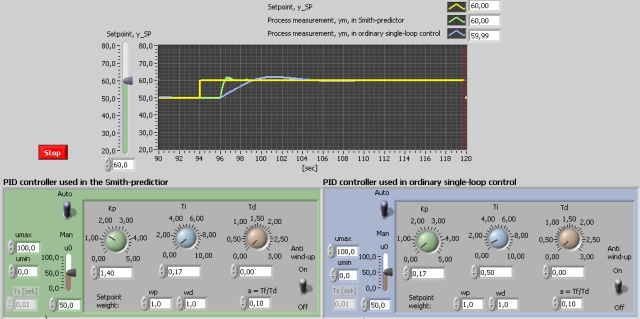
Snapshot of a part of the front panel of the simulator:

- What is needed to run the the simulator? Read to get most recent information!
- Tips for using the simulator.
- The simulator: smith_predictor.exe . The simulator runs immediately after the download by clicking Open in the download window. Alternatively, you can first save a copy of the exe-file on any directory (folder) on your PC and then run the exe-file, which starts the simulator.
Description of the system to be simulated
This simulator simulates a control system based on the Smith-predictor, which implemenets dead-time compenastion. The process to be controlled is given as a transfer function model of the form "first order system with dead-time". For clear comparison a traditional single-loop control system for an identical process is simulated in parallell.
The Smith-predictor contains a PID-controller. In the simulator there is support for tuning this controller as a PI-controller based on pole-placement design [cf. Ch. 8 in PID Control (to appear during Summer 2004)].
In the simulator the PI(D)-controller in the traditional single-loop control system can be tuned as a PI-controller using Skogestad's method of PID-tuning [cf. Ch. 8 in PID Control (to appear during Summer 2004)].
Aim
To see the benefits and drawbacks of using Smith-predictor to control processes having dead-time compared to using ordinary single-loop control.
Motivation
Some industrial processes has a dominating dead-time, e.g. transportation processes. Using ordinary single-loop PID control the dead-time forces the bandwidth of the control system to be relatively low. If the dead-time can not be reduced, usning a Smith-predictor may be beneficial both for tracking control purposes and disturbance compensation purposes.
Tasks
If nothing else is stated, you should use the default values of the parameters (in general, the default value is retrieved using right-click in the element on the front panel of the simulator).
- Assuming perfect process model:
Use the following parameters in both the process model
and the process model usind internally in the Smith predictor: Ku
= 1 = Kv, T = 0.5 sec and tau = 2 sec (relatively large dead-time).
Thus, there is no model errors in this case.
- Tune the PI controller in the Smith-predictor and the PI controller in the traditional single-loop control system. (Alternatively, you can use the following parameters: Smith-predictor: Kp = 1.4 and Ti = 0.17. Traditional single-loop control system: Kp = 0.17 and Ti = 0.50.)
- Check (using simulations) if the tracking properties and the distrurbance compensation properties are better with the Smith-predictor than with traditional single-loop control system. In the simulations you can apply setpoint steps and disturbance steps, respectively.
- Robustness of Smith-predictor against model
errors: Use the same parameter values as in Task 1,
unless otherwise stated (below).
- Increase the dead-time of the controlled process from 2.0 to 2.5 sec (without adjusting any controller parameter). Is the Smith-predictor robust against this parameter change, which introduces a model error. (Observe the stability of the control system). What about the traditional control system - does it have greater robustness against the model error?
- Are the two stability of each of the two control systems robust against a reduction of the dead-time from 2.0 to 1.5?
- Improving the robstness of the
Smith-predictor?:
- Tune the PI controller in the Smith-predictor out from the following more careful or conservative requirement: The relative damping factor, z, of the internal control loop in the Smith-predictor is increased from 0.6 to 0.8, and, in addition, the natural resonance frequency, w0, is reduced to the half, from 4 to 2 rad/s. (Alternatively, you can use the following PI parameters in the Smith-predictor: Kp = 0.6 and Ti = 0.3 sec.)
- Check if the robustness of the Smith-predictor is improved as compared to Task 2.
Updated 21. January 2008. Developed by Finn Haugen. E-mail: finn@techteach.no.
