|
|
Guidelines to
PID Control with
LabVIEW
by
14. November 2008
Introduction
Installing the PID Control Toolkit, also named Control Toolkit, or the Real-Time Module adds the PID Palette to the . It is also avaible on the in LabVIEW. The PID Palette has a number of functions for PID control applications.
It seems to me to be a need for some guidelines - both for students and engineers - for using the PID control function(s) on the PID Palette correctly. The purpose of this document is to give such guidelines.
This tutorial is based on LabVIEW 8.5.
Let us start with taking a look at the PID Palette.
The PID Palette
The figure below shows the functions of the PID Palette.
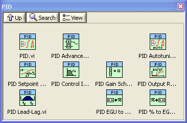
The PID Palette
A few comments to the functions on the Control Palette:
-
The PID function implements a PID controller function on the summation (or parallel) form. The PID function implements anti-windup. It has no lowpass filtering in the derivative term, so the derivative term may give very high amplification of high-frequent measurement noise. It can not be set in manual mode, making it a little difficult to use in tuning and startup, and therefore I do not use this PID function, but the next one.
-
The PID Advanced function implements a PID controller function on the summation form, i.e. the P, I, and D terms are summed, and with controller parameters Kc, Ti and Td. (More precisely, the summation form realizes the so-called ideal form of the PID controller function. The other summation form is the parallell form with controller parameters Kc, Ki = Kc/Ti, and Kd = Kc*Td.) The PID function implements anti-windup, and it can be set in manual mode. Options are nonlinear gain and reduced setpoint weight in the proportional term (these options are not well documented). It has no lowpass filtering in the derivative term. (In applications I always use the PID Advanced function, not the PID function, due to the lack of the manual mode option in the latter.)
-
The PID Autotuning function implements an autotuner based on the Relay method. (In the tuning phase a Relay function acts as an On/Off controller, causing sustained oscilllations in the control loop. Information about these oscillations are used to calculate proper PID settings.)
-
The PID Setpoint Profile function can be used to define a profile of the setpoint time function based on piecewise constant and/or linear increasing/decreasing, i.e. ramped, time functions. The ramps provides a smooth change between two setpoint values.
-
The PID Control Input Filter function is a 5'th order FIR filter which can be used to smooth the measurement signal. Of course, other filtering functions can be used, too, e.g. the Butterworth Filter PtByPt function on the .
-
The PID Gain Schedule function implements gain scheduling of the PID parameters based on a piecewise constant interpolation of a given set of PID settings. You can use as many different sets of PID settings as you want in the gain (or PID parameter) schedule.
-
The PID Output Rate Limiter function limits the rate of change of the PID controller output, i.e. the calculated control signal.
-
The PID Lead-Lag function implements a transfer function with a first order numerator and a first order denominator. It can be used in feedforward control, and possibly in a decoupler in a multivariable controller.
-
The PID EGU to % function can be used to scale a measurement signal from engineering unit to percent.
-
The PID % to EGU function can be used to scale the calculated PID control signal from percent to engineering unit, e.g. ampere or voltage.
Using the PID Advanced function
Here the PID Advanced function is described, not the PID function which seems to be just a simpler version of the PID Advanced, lacking the important feature of setting the controller in manual mode.
Below is the Front panel and the Block diagram of pid_control_labview.vi, which is in the zip-file pid_control_labview.zip (together with the lowpass filter timeconstant_lowpass_filter.vi) which implements a PID speed control loop for a simulated motor having gain 0.5 and time-constant 2 sec (the model is represented with a transfer function). This model includes the speed sensor. In the simulator random measurement noise is included to make the simulator more realistic. This simulator is ready to run if you have the LabVIEW Simulation Module installed. Click on the figures to see them in full sizes.
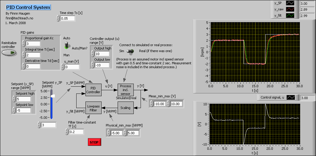
Front panel of pid_control_labview.vi (which is in the zip-file pid_control_labview.zip)

Block diagram of pid_control_labview.vi (which is in the zip-file pid_control_labview.zip)
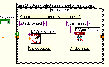
In Case Structure - Selecting simulated or real process in the upper-right part of the block diagram the True case can be as shown in the figure below (in the downloadable pid_control_labview.vi the True case does not contain the DAQmx Write and DAQmx Read functions).
Here are comments to pid_control_labview.vi:
- On the PID Advanced function: Auto/Man? is used to set the PID controller in either manual mode or automatic mode.
- u_man is the value of the control signal when the controller is in Manual mode. The value has no effect when the controller is in Automatic mode.
- Output range (a cluster) defines the maximum and minimum value of the PID control signal. It is important to set these values correctly, otherwise the important anti windup feature will not work properly.
- Reinitialize controller is used to set the internal variables of the PID function back to the default values. For example, the integral term is reset.
- Setpoint is the desired value of the process measurement signal.
- Sepoint range (a cluster) defines the maximum and minimum value of the setpoint. It is important to set these values correctly, since they are used in the implementation of the anti windup feature.
- PID gains (a cluster) contains the three PID parameters. The input to the PID Advanced function assumes that Ti (integral time) and Td (derivative time) are in minutes. However, in many (most?) applications it is more convenient to let the user adjust Ti and Td in seconds. The Block diagram implements the transformation from seconds to minutes using the Cluster PID Scaling from Sec to Min together with a Divide function. If you want to keep minute as time unit just remove the latter cluster and the Divide function, and wire PID gains directly to the PID Advanced function.
- Time step Ts is wired to the dt of the PID Advanced block. It is the time step of the controller, and it is one of the parameters of the function. It has to have the same value as the actual time step of the execution of the PID Advanced function, which in our VI means that it has to have the same value as the While loop cycle time. If you do not wire any value to the dt in put, the PID Advanced function is actually able to detect the actual time step itself. However, I suggest that you define the time step explicitly, as shown in the Block diagram. (When using the PID Advanced function in a Simulation Loop, as in the present VI, you have to define the dt input explicitly to be sure the PID function works correctly.)
-
A measurement lowpass filter in the form of the sub-VI timeconstant_lowpass_filter.vi is included to attenuate the inevitable high-frequent measurement noise that exists in all practical control systems. (This noise will be transferred to the actuator via the controller, and may cause excessive wear on.a mechanical actuator as a motor, a relay, etc.)
The PID control palette contains a measurement filter in the form of a fifth order lowpass FIR filter, see the Control Palette, but this filter can not be tuned.
LabVIEW has lots of filtering functions, but the advantages of timeconstant_lowpass_filter.vi compared to these is that the filter parameter (time constant) can be changed online without the filter output being reset to zero, and that the initial filter output equals the initial filter input (thereby avoiding the initial filter output to be zero). - Polynomial Interpolation functions have been used to scale the measurement signal (assumed to be voltage) to a scaled value (assumed to be percent) and to unscale the PID controller ouput signal (assumed to be in percent) to the raw or physical control signal (assumed to be voltage) to be sent to the actuator. There are (un)scaling functions on the PID Control palette, too, see end of PID Control Palette Section above. These functions assume percent to be one of the units, while the Polynomial Interpolation function can be used with any units.
In a practical application you may use the pid_control_labview.vi as the starting point. You may keep the Simulation Loop, but if you want, you may substitute the Simulation Loop with a While Loop or Timed Loop, but if you do, you must remove the Simulation Module functions (as the Transfer Function and the Simulation Time Waveform) since they can not be used other loops than the Simulation Loop.
Note the following if you use the PID Advanced function in a Simulation Loop: You must force the PID Advanced function to be invoked only at the major time steps of the simulator, otherwise the function may not behave correctly. This is done as follows: Right-click on the PID Advanced function / Select SubVI Node Setup / Select Continuous and deselect Include minor time steps.