Discrete-Time PID Controller

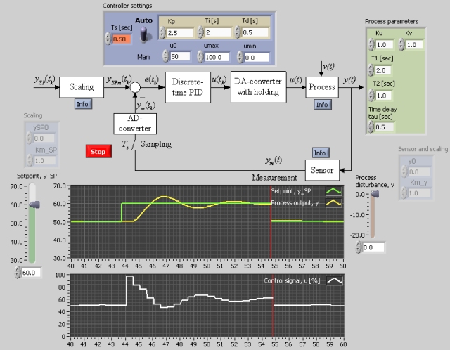
Snapshot of the front panel of the simulator:

• What is needed to run the the simulator? Read to get most recent information!
• Tips for using the simulator.
• The simulator: piddiscrete.exe . The simulator runs immediately after the download by clicking Open in the download window. Alternatively, you can first save a copy of the exe-file on any directory (folder) on your PC and then run the exe-file, which starts the simulator.

Description of the simulated system

Typically, commercial PID controllers of today are implemented as an algorithm running on a computer. The PID algorithm is executed once per time step (sampling interval), Ts. A typical value of Ts is 0.1 sec. The tasks below deomonstrates effects of the discrete-time nature of such computer implemented controllers.

Tasks

Assuming the following parametrers of the process to be controlled (these values are default values of the simulator): Ku=1, Kv=1, T1=2, T2=1, tau=0.5. Controller tuning using the Ziegler-Nichols' ultimate gain tuning method yields

Kp=3.6, Ti=2.0 og Td=0.5

You can apply the above parameter values in the following task.

Start the simulator.

1. Set Ts =  0.1. Change the setpoint e.g. as a step. Observe the control signal. Does this signal seem to be almost continuous?
2. Increase Ts to 0.5. What does the control signal look like? What has happened to the stability of the control system?
3. Find experimentally (on the simulator) for which values of Ts the control system is asymptotically stable.
4. Adjust Ts to the value giving marginally stability of the control loop. Readjust the PID parameters so that the loop again becomes asymptotically stable (using e.g. the Ziegler-Nichols' closed loop method). Is the control loop as quick with this new PID setting as with the original setting?

[SimView] [TechTeach]

Updated 2 September 2017. Developed by Finn Haugen. E-mail: finn@techteach.no.