![]()
Temperature Control of Liquid Tank
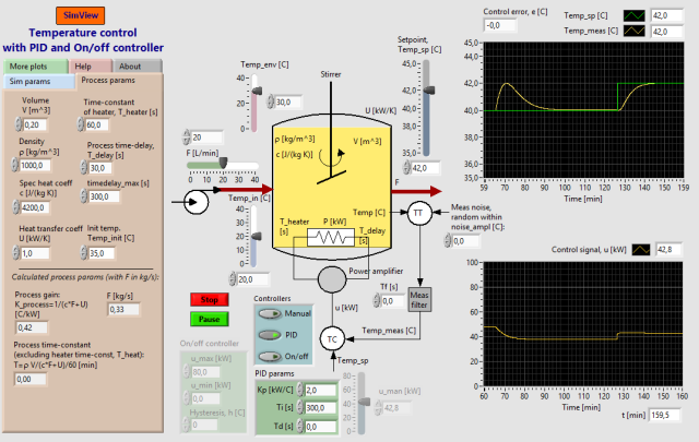
Snapshot of the front panel of the simulator:
- What is needed to run the the simulator? Read to get most recent information!
- Tips for using the simulator.
- The simulator: temp_control_pid_onoff.exe.
Description of the simulated system
A temperature control system for a water tank with continuous inflow and outflow is simulated. The water is heated by a heating element which controlled by the controller. The temperature is measured by a temperature sensor which in practice may be a Pt100 element or a thermocouple.
The process model on which the simulator is based is a 1. order model based on energy balance under the assumption of homogenous conditions in the liquid in the tank. The processs model also contains a time delay which represents the time delay which in practice exists between an exitation of the heating element and the response in the temperature sensor. In addition the simulator contains a 1. order transfer function representing a time constant in the heating element.
Video
Here are some instructional videos where the present simulator is used as an example:
- PID controller tuning with the Good Gain method
- PID controller tuning with Ziegler-Nichols' oscillations method
Process model
Knowledge about the process model is not necessary for doing the tasks below. The parameter values are shown on the front panel of the simulator.
The process model used in the simulator is based on energy balance:
(1) d(crVT1)/dt = Keu + cw(Tinn - T1) + U(Tenv - T1)
where Keu = P is the power delivered by the heating element. T1 is the temperature in the tank assuming homogenous conditions. In practice there is a time delay between an excitation in the heating element and the response in the temperature sensor:
(2) T(t) = T1(t-t)
We assume that this time delay is inversely proportional to the mass flow w:
(3) t = Kt/w
By taking the Laplsce transform of the model above we can get the following transfer function from the control signal to the temperature T:
(4) T(s)/u(s) = H(s) = [Ku/(Ts+1)]e-ts
Thus a first order model with time delay. The parameters of H(s) are:
(5) Gain Ku = Ke/(cw+U)
(6) Time constant Tk = rV/(w+U/c)
(7) Time delay t = Kt/w
In addition the simulator contains a 1. order transfer function representing a time constant in the heating element. (This submodel is not shown in the model above.)
Aims
- To get an understanding of how an automatic control system based on feedback works and which benefits feedback control has compared to control using a constant control signal.
- To get an understanding of the features of the PID controller and the on/off controller.
- To get skills in tuning a PID controller
- To get insight into the importance of different system parameters on the dynamic properties of the control system.
In other words: You will get knowledge about the basics of control!
Motivation
Control systems are essential in industrial processes since it is important and useful to control process variables so that they are kept on or close to specifies values (setpoints). The PID controller is the most frequently used control function in industrial systems.
In the industry temperature control is used on e.g. reactors and heat exchangers.
Tasks
The nominal operating point of the process is defined as follows:
- The tank temperature T is 50 degrees C.
- The inlet temperature Tin is 20 degrees C.
The default process parameter values are as shown on the this snapshot of the front panel of the simulator.
Unless otherwise stated it is assumed that the tasks below are executed while the simulator runs.
- First: Control using constant control
signal. Set the controller in manual mode.
Find the nominal control signal uman "experimentally". Then
change the distrubance Tin from 20 to 15 degrees C. What is
the value of the resulting steady-state control error?
- Feedback control by you
! Reset the settings of the simulator to its default
values (menu: Operate / Reinitialize All to Default), but the controller
shall be in manual mode.
Change the disturbance Tin from 20 to 15 degrees C, and
control the process via the nominal control signal u0. Are
you able to obtain zero steady-state control error?
- Automatic control using a PI
controller: Tuning the controller: Tune the controller
using the Ziegler-Nichols' closed loop method.
In the subsequent tasks you shall use a PI controller with settings as found in Task 4. Alternatively, you can use the following parameter values:
Kp = 2.6, Ti = 6.3 min, Td = 0s
-
Disturbance compensation:
Reset the settings of the simulator to its default values (menu:
Operate / Reinitialize All to Default). Change the disturbance Tin
from 20 to 15 degrees C. What is the steady-state control error?
- Setpoint tracking:
Change the setpoint as a step, say from 50 to 60 degrees C. What is the
steady-state control error?
- The stability of the control system at parameter
variations:
Reset the settings of the simulator to its default values (menu: Operate
/ Reinitialize All to Default). Check what happens with the stability of
the control system at the below parameter changes. In each of the
subtasks/experiments you can excite the control system using a
small step in the setpoint. The experiments shall be performed
independent of each other, that is, the parameters should be reset to
the default values once the experiment is completed.
- Controller gain Kp is increased (much).
- Integral time Ti is reduced (much).
- Derivative time Td is increased (much).
- Power gain Ke is increased (much).
- Mass flow w is decreased (much).
- Measurement gain Km,TT is increased (much). (This gain is the ration between the temperature measurement in % and the temperature in degreees C. The gain is changed by changing the measurement range. If you change the measurement range, you must also change the setpoint range accordingly, otherwise there will be a steady-state control error.)
Updated 2 September 2017. Developed by Finn Haugen. E-mail: finn@techteach.no.