 |
|
Introduction
to simulation with
Control Design and
Simulation Module
in LabVIEW 8.6
by
16. March 2009
Contents:
1 Preface
2 Introduction
3 The contents of the
Simulation functions palette (Video)
4 An example:
Simulator of a liquid tank
4.1
Developing the mathematical model of the system to be simulated
4.2 The
Front panel and the Block diagram of the simulator
(Videos)
4.3
Configuring
the simulation
(Videos)
5 Various topics
5.1
Representing state space models using Formula node and integrators
5.2 Creating subsystems
5.3 Getting a linearized model of a subsystem
5.4
Simulating control systems
5.5 Converting models between Simulation Module and Control Design Toolkit
5.6
Putting code into a While loop running in parallell with a Simulation loop
5.7 Translating SIMULINK models into LabVIEW Simulation models
1 Preface
This document gives an introduction to the simulation tools of the LabVIEW Control and Simulation Module for LabVIEW 8.6. It is assumed that you have basic skills in LabVIEW programming. There are tutorials for LabVIEW programming available from the National Instruments' webside http://ni.com, and I have made one myself (to serve the needs in my own teaching more specifically), see Finn's LabVIEW Page.
This tutorial contains a number of activities that you are supposed to perform. These activities are shown in blue boxes, as here:
| Activities are shown in blue boxes as this one. |
Most of the activities are video-based. In the former tutorial, based on LabVIEW 8.5, there were no videos, but in stead detailed explanations. I have removed the explanation in the present tutorial where the videos give the same information.
If - for some reason - the videos does not display correctly in the current player, try some other. Windows Media Player is probably the default video player on your PC. Alternative players are RealPlayer and QuickTime (both can be downloaded from the Internet for free).
More tutorials that may be relevant for you as a LabVIEW user are available from Finn's LabVIEW Page.
2 Introduction
The LabVIEW Control and Simulation Module contains a block diagram based environment for simulation of linear and nonlinear continuous-time and discrete-time dynamic systems. Many simulation algorithms (i.e. numerical methods for solving the underlying differential equations) are available, e.g. various Runge-Kutta methods. The mathematical model to be simulated must be represented in a simulation loop, which in many ways is similar to the ordinary while loop in LabVIEW. You can make the simulation run as fast as the computer allows, or you can make it run with a real or scaled time axis, thus simulating real-time behaviour, with the possibility of the user to interact with the simulated process. The simulation loop can run in parallel with while loops within the same VI.
3 The contents of the Simulation functions palette
Once the Control and Simulation Module is installed, the Simulation palette is available from the Functions palette. The video below gives overview over the contents of the Simulation Palette.
| Play the video sim_palette_overview (17 minutes, the video will be opened in a new window) to get an overview over the contents of the Simulation Palette. It is assumed that you have the block diagram of any VI opened. |
4 An example: Simulator of a liquid tank
In this section we will study and partly develop a simulator of a liquid tank. Actually, we will play with a premade example, but not develop it from scratch. I think this is an effective way to learn using the tools, assuming that you have basic skills in LabVIEW programming. You are supposed to have basic knowledge about modeling of dynamic systems, as described in e.g. Dynamic Systems - modelling, analysis and simulation or in any other book about dynamic systems theory.
4.1 Developing the mathematical model of the system to be simulated
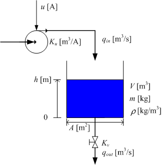
The system to be simulated is a liquid tank, see the figure below. The simulator will calculate and display the level h at any instant of time. The simulation will run in real time, with the possibility of scaled real time, thereby giving the feeling of a "real" system. The user can adjust the inlet by adjusting the pump control signal, u.
Liquid tank
Any simulator is based on a mathematical model of the system to be simulated. Thus, we start by developing a mathematical model of the tank.
We assume the following (the parameters used in the expressions below are defined in the figure above):
- The liquid density is the same in the inlet, in the outlet, and in the tank.
- The tank has straight, vertical walls.
- The liquid mass and level are related through
m(t) = ρAh(t)
- The inlet volumetric flow through the pump is proportional to the pump
control signal:
qin(t) = Kuu(t)
- The outlet volumetric flow through the valve is proportional to the square
root of the pressure drop over the valve. This pressure drop is assumed to be
equal to the hydrostatic pressure at the bottom of the tank (sqrt means square
root):
qout(t) = Kvsqrt[ρgh(t)]
Mass balance (i.e., rate of change of the mass is equal to the inflow minus the outflow) yields the following differential equation:
dm(t)/dt = ρqin(t) - ρqout(t)] (1)
or, using the above relations,
d[ρAh(t)]/dt = ρKuu(t) - ρKvsqrt[ρgh(t)] (2)
We will now draw a mathematical block diagram of the model. This block diagram will then be implemented in the block diagram of the simulator VI. As a proper starting point of drawing the mathematical block diagram, we write the differential equation as a state-space model, that is, as a differential equation having the first order time derivative alone on the left side. This can be done by pulling ρ and A outside the differentiation, then dividing both sides by ρA. The resulting differential equation becomes
d[h(t)]/dt = (1/A)*{Kuu(t) - Kvsqrt[ρgh(t)]} (3)
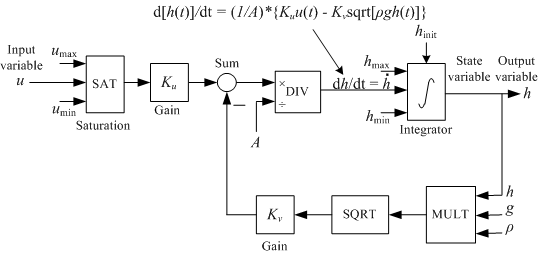
This is a differential equation for h(t). It tells how the time derivative dh(t)/dt can be calculated. h(t) is calculated (by the simulator) by integrating dh(t)/dt with respect to time, from time 0 to time t, with initial value h(0), which we here denote hinit. To draw a block diagram of the model (3), we may start by adding an integrator to the empty block diagram. The input to this integrator is dh/dt, and the output is h(t). Then we add mathematical function blocks to construct the expression for dh/dt, which is the right side of the differential equation (3). The resulting block diagram for the model (3) can be as shown in the figure below.
Mathematical block diagram of Differential Equation (3)
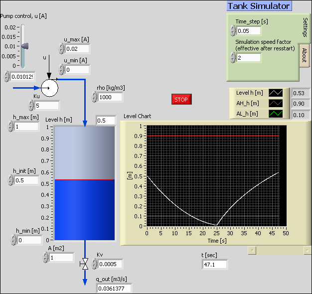
The numerical values of the parameters are shown in the front panel picture below.
We will assume that there are level alarm limits to be displayed in the simulator. The limits are
AH_h = 0.9m (Alarm High)
AL_h = 0.1m (Alarm Low)
The block diagram developed above will be implemented in a Simulation Loop in the Block diagram of our simulation VI.
4.2 The Front panel and the Block diagram of the simulator
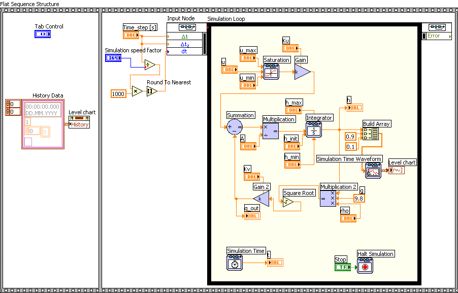
The subsequent figures show the front panel and the block diagram of the complete VI, tanksim.vi.
Front panel of tanksim.vi.
Block diagram of tanksim.vi.
The Front panel
|
Open the Front panel of
tanksim.vi. Play the video tanksim_frontpanel (20 minutes, the video is opened in a new window) to |
The Block diagram
|
Open the Block diagram of
tanksim.vi. Play the video: tanksim_blockdiagram (42 minutes, the video is opened in a new window). Note: In the beginning of the video I refer to four videos, but I have compiled these four videos into one video. |
4.3 Configuration of the simulation
|
Play the video
tanksim_config_sim (28 minutes, the video is opened in a new window). Note: In the video a figure illustrating the time step (or step size) is shown. In the video I say that this figure exists in the tutorial, but it does not (but you see it in the video). |
5 Various topics
(There are no blue activity boxes in Chapter.)
5.1 Representing state space models using Formula node and integrators
A state-space model is a set of first order differential equations constituting the model of the system. State-space models is a standardized model form. It is common that mathematical models of dynamic systems are written as state-space models. To be a little more specific, here is a general second order state-space model (the dots represents the arguments of the functions):
dx1/dt = f1(x1,x2,...)
dx2/dt = f2(x1,x2,...)
y = g(x1,x2,...)
where f1(•) and f2(•) are functions containing the right-hand part of the first order differential equations. The arguments may be state variables, input variables, and parameters. These functions may be linear or nonlinear. They are the time-derivatives of the states, x1 and x2, respectively. Sometimes one or more output variables are defined. Above, the output variable is y, and the output function is g(•).
To implement the block diagram of a state-space model, you may start by adding one Integrator block for each of the state variables on the block diagram. The output of the integrators are the state variables. The inputs to the integrators are the time derivatives, and the f1(•) and f2(•) functions in the representative model shown are these time derivatives. To implement the functions you have the following two options (which also may be combined):
- Constructing the functions, f1(•) and f2(•) above, using block functions as Sum, Gain, Multiplication etc., which are on the Simulation Palette of the Functions Palette. One example is the Block diagram of the model of the liquid tank shown here.
- Writing the textual functions of f1(•) and f2(•) in a Formula Node. The Formula node is on the Mathematics / Scripts & Formulas Palette (and on the Structures Palette). The Formula Node is explained here (in my Introduction to LabVIEW). With the Formula Node the functions are easier to modify (it is done by justing editing text in the Formula Node), and the Block Diagram may appear simpler. However, it may be difficult to implement nonlinear functions as hysteresis, backlash etc. (there are numerous such nonlinear blocks in the Nonlinear Palette on the Simulation Palette).
Here is a simple example of using the Formula node. Given the following state space model:
dx1/dt = x2
dx2/dt = -x1 + u
y = x1
(which is a state space model of an oscillator). u is the input variable, and y is the output variable. ssformulanode.vi shown below implements a simulator for this system. A Formula node is used to represent the right side of the differential equations. The integration of the time derivatives are performed by Integrator blocks from the Continuous palette.
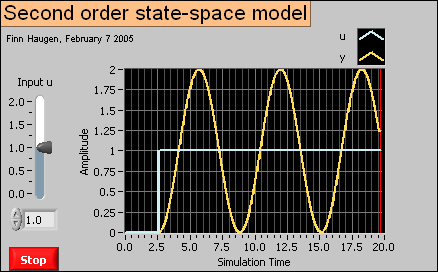
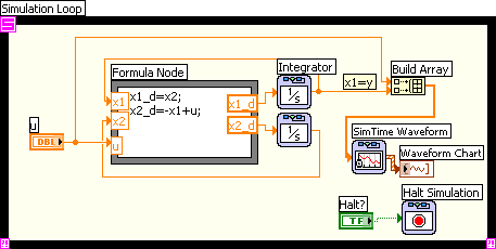
Front panel and block diagram of ssformulanode.vi.
Using Formula Node in stead of block functions to calculate the time derivatives may give a simpler block diagram. However, if the expressions for the time derivatives (i.e. the right-hand sides of the differential equations) contains nonlinear functions, it may be more difficult to implement these in the Formula Node than with function blocks.
5.2 Creating subsystems
You can create a subsystem of a part of a simulation diagram. The first step is to select or mark the part of interest, see the figure below, which shows the block diagram of tanksim.vi.
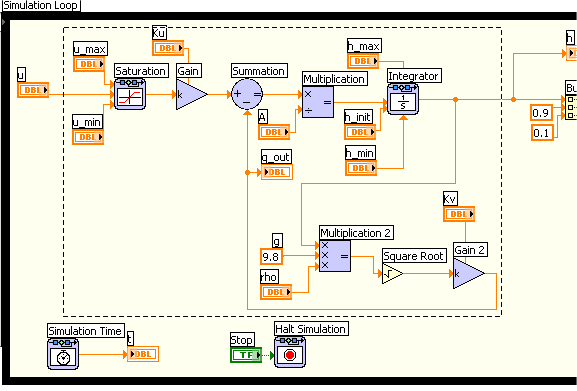
The first step in creating a subsystem in the simulation diagram is to select the part of interest
Then the subsystem is created using the menu . The resulting diagram is shown in the figure below.
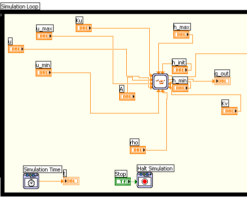
The resulting simulation diagram, including the subsystem
Note that you can change the size of the subsystem icon using the cursor.
If you want you can open the front panel of the subsystem by double-clicking the subsystem icon, see the figure below.
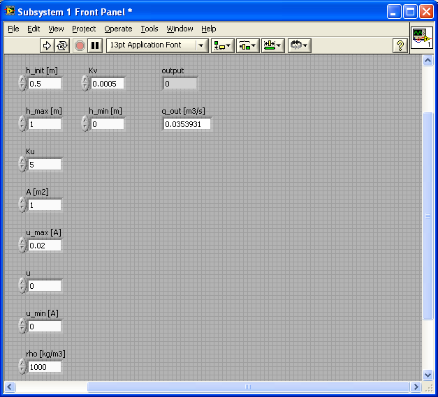
The front panel of the subsystem
You can open the block diagram of the subsystem via the menu, see the figure below.
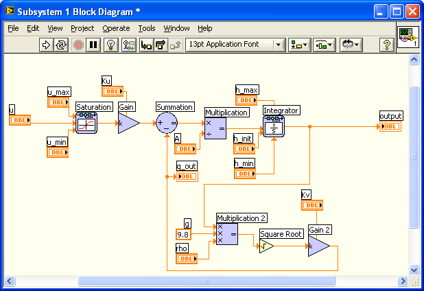
The block diagram of the subsystem
5.3 Getting a linearized model of a subsystem
LabVIEW can create a linear state space model from a linear or nonlinear subsystem. (Creating subsystems is described in the previous section.) The procedure is to select or mark the subsystem of interest, and then create the linear model by using the following menu: . You are given the option of saving the linear model as a model (to be used by functions in the Control Design Toolkit) or as a VI containing the state space model in the form of a cluster of coefficient arrays. Perhaps the most flexible choice is VI.
5.4 Simulating control systems
Simulating control systems is done in the same way as simulating dynamic systems. You can include virtually every control function in a model block diagram inside the Simulation Loop. In Guidelines to PID Control with LabVIEW there is an example of a simulator of a PID control system.
5.5 Converting models between Simulation Module and Control Design Toolkit
You can convert models between the Simulation Module and the Control Design Toolkit using the conversion functions on the Model Conversion palette on the Control Design Tookit. The two conversion functions are shown in the figure below.
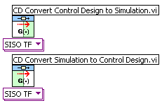
The conversion functions on the Control Design Toolkit / Model Conversion palette
5.6 Putting code into a While loop running in parallell with a Simulation loop
It is possible to put almost any LabVIEW code for e.g. analysis and design of into a simulation diagram inside a Simulation loop, but doing so may give an unnecessary large or complicated simulation code, and the simulation execution may be delayed. Therefore, you should not put more code inside the Simulation loop than is strictly necessary for representing the model to be simulated. Other parts of the total code, e.g. optimal control design functions (as the LQR function) or Kaman filter (state estimator) design functions (as the Kalman Gain function), may be put into one or more ordinary While loops running in parallel with the Simulation loop. These While loops may be programmed to run slower than the Simulation loop. Data can be exchanged between the loops using local variables (local variables are described in Introduction to LabVIEW).
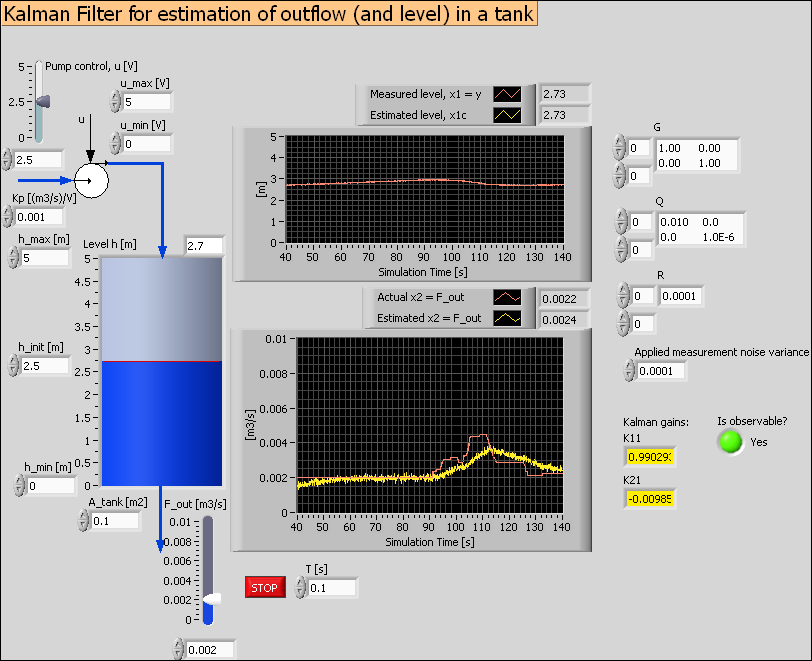
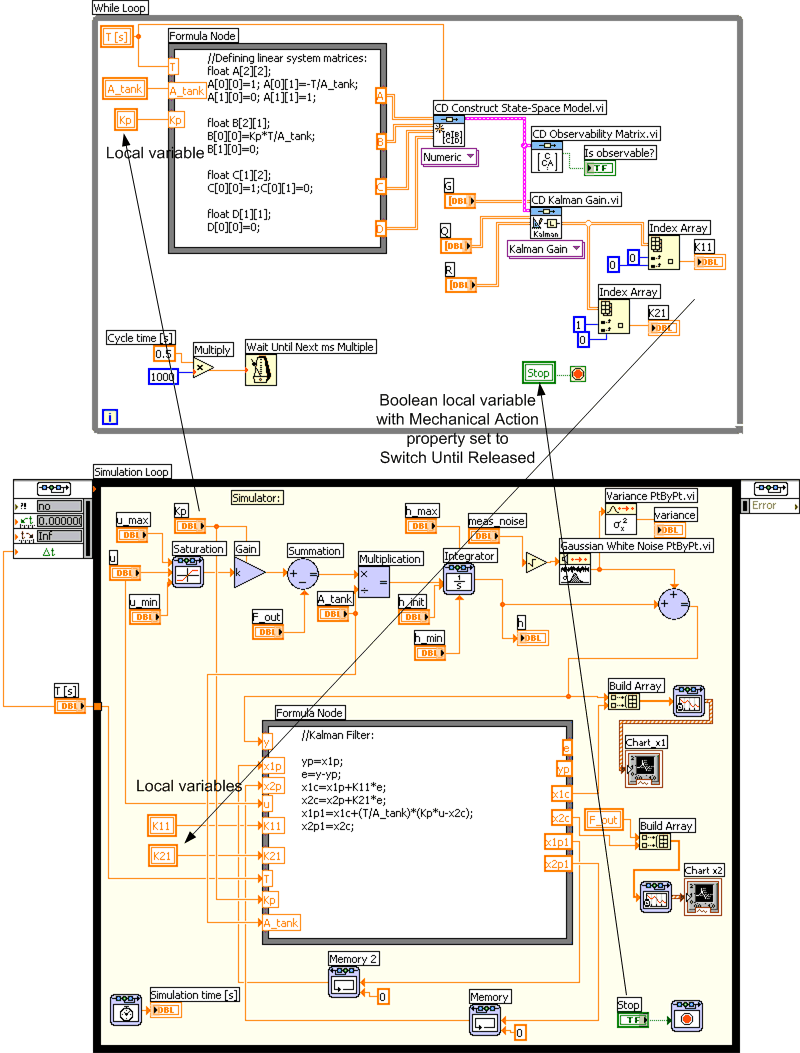
Here is one example: kalmanfilter_tank.vi is a simulator of a Kalman Filter which estimates the outflow of a simulated liquid tank. (You can run this simulator if you have the LabVIEW Simulation Module installed.) The simulator is implemented with a Simulation Loop which contains a model of the tank and the expressions constituting the Kalman Filter algorithm. The Kalman gains are calculated using the Kalman Gain function of the Control Design Toolkit. This function is relatively computational demanding, and it is therefore put into a While loop which runs in parallell with the Simulation loop with a cycle time of 0.5 sec. The Kalman gains are made available inside the Simulation loop using local variables.
The simulation time step is 0.1 sec, and the Period (which is the actual, real time that LabVIEW used to proceed one simulation time step) is 0.025 sec. (Having the Period smaller than the simulation time step makes the simulator run faster than real time. This is favourable here since the process itself is a slow system, and we do not have time to sit waiting for responses to come.) If we had put the Kalman Gain function inside the Simulation loop, the specified Period of 0.025 sec could not have been obtained because it takes about 0.3 sec (this is however computer-dependent) to execute Kalman Gain function.
Below are the front panel and the block diagram of kalmanfilter_tank.vi. Click on the figures to see them in full sizes. Note how local variables are used to exchange values across the loops. Note also how the Stop button and its local variable is used to stop both loops. The Mechanical Action property of the Stop button must be set to Switch until Released. If it is set to one of the Latch... properties, it it will not be possible to create local variable for it.)
Front panel of kalmanfilter_tank.vi (click on the figure to see it in full size)
Block diagram of kalmanfilter_tank.vi (click on the figure to see it in full size)
5.7 Translating SIMULINK models into LabVIEW Simulation Module models
You can translate SIMULINK (MathWorks) models into LabVIEW simulation models using the menu Tools / Simulation Tools / SIMULINK Translator in LabVIEW.
