Examples of Student Assignments on Modeling, Simulation, and Control

This document and the linked files are available at http://techteach.no/presentations/. (The files may be updated at any time.)

Contents of this document

1 Introduction
2 Hardware-in-the-loop simulation
3 Implementation of PID controller function from scratch
4 Mathematical modeling of physical processes
5 Simulation of physical processes and its control system
6 State estimation using Kalman Filter algorithm

1 Introduction

1.1 A few words about my background

A few words about my background (http://techteach.no):

• Teaching and writing and consulting in control engineering since about 1990
• Associate Professor (80% position) at Telemark University College and consultant via TechTeach
• Developing KYBSIM (http://techteach.no/kybsim) - a library of freely available simulators developed in LabVIEW for dynamic systems, control and signal processing
• Using LabVIEW extensively in teaching (simulators and student assignments). Creating measurement and control applications in research applications.

[Contents]

1.2 Outline of the presentation

Presentation description

The author has been teaching mathematical modeling, simulation and control for about 20 years in both bachelor and master studies. Here he presents and gives demonstrations of some successful students assignments within this area. Theory and practice are combined in an efficient way thanks to powerful graphical software tools which are well integrated with I/O hardware connected to physical processes. This efficient combination of theory and practice motivates and enhances students teaching. In the assignments presented, hardware and software tools by National Instruments’ are used.

Let us take a look at a number of student assignments!

[Contents]

2 Hardware-in-the-loop (HIL) simulation

Example of HIL-simulation: A Fuji PYX5 PID controller controls a simulated first order plus time-delay process

At Buskerud University College the students develop a system for hardware-in-the-loop simulation:

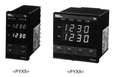
Fuji PYX5 Process Controller

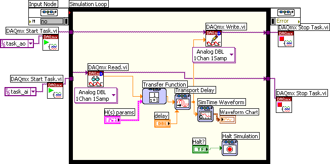
The Fuji controller controls a simulated process. The simulator runs in real time and is implemented in LabVIEW Simulation Module running on a PC:

PC with LabVIEW Simulation Module

The analog control signal from the Fuji controller controls the simulated process via one of the analog input channels on the USB-6008 device, and the simulated process measurement signal is connected to the controller via one of the analog output channels on the USB-6008 device.

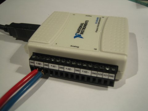
USB-6008 device

Here is the simulator:

[Contents]

Example of HIL-simulation: A Simatic PLC controls a simulated drill

Master student Tommy Andersen (Telemark University College) now implements the following HIL system which we hope to use in PLC courses:

Simatic PLC (S7-300)

Front panel of simulated drill implemented in LabVIEW Simulation Module on a PC:

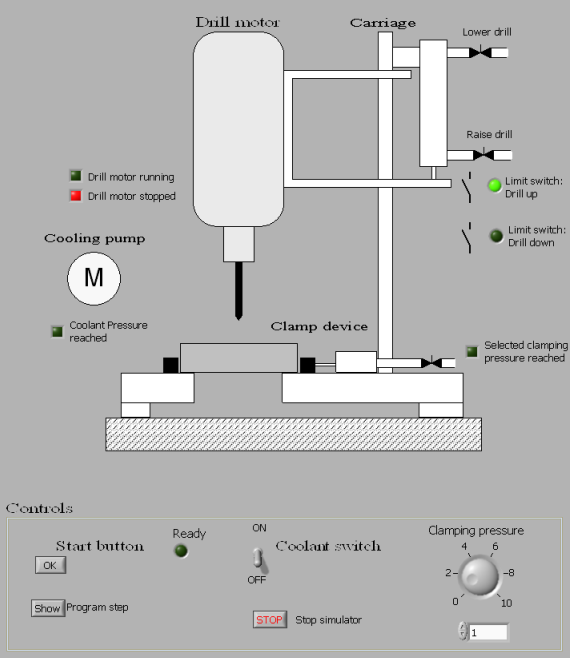
Simulated drill

Sequential control program implemented in Graph7 in the PLC:

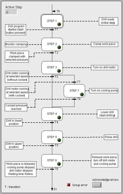
Sequential control program implemented in Graph7

The PLC and the PC with LabVIEW drill simulator communicates using OPC (OLE for Process Control), see the figure below:

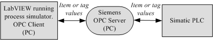
OPC based communicatioin between LabVIEW and Simatic PLC

[Contents]

3 Implementation of PID controller function from scratch

Example: Implementation of a practical PI(D) controller function

In the master study at Telemark University College the students implement a practical PI(D) controller having

• Auto/manual options
• Anti-windup
• Direct/reverse action
• Bumpless transfer
• Lowpass filter in the derivative term

The controller is implemented in Formula Node in LabVIEW:

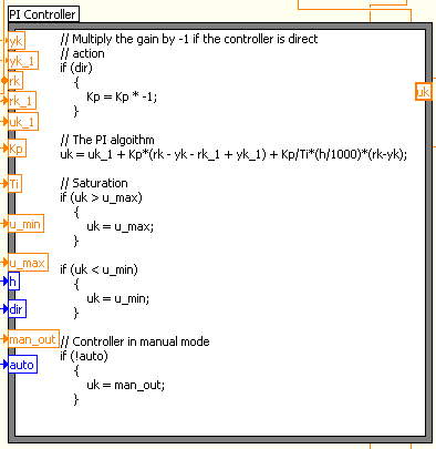
Student's PI controller

The PID controller is tested against both a simulated and a real process.

[Contents]

4 Mathematical modeling of physical processes

Example: Modeling of a liquid tank

At Telemark University College students develop two different kinds of mathematical models of the liquid tank shown below:

• A differential equation based on mass balance of the water in the tank:

  dy/dt = K₁*u - K₂*sqrt(y)

  
  The model estimation (i.e. calculation of K₁ and K₂ can be made using e.g. by doing some clever experiments or by applying the least square method.
   

• A discrete time transfer function (from pump control signal to water level measurement signal):

  H(z) = y(z)/u(z)

  The model estimation is based on the subspace Estimate State-Space Model function available in the System Identification Toolkit.

  The figure below shows how the Estimate State-Space Model function can be used.

  

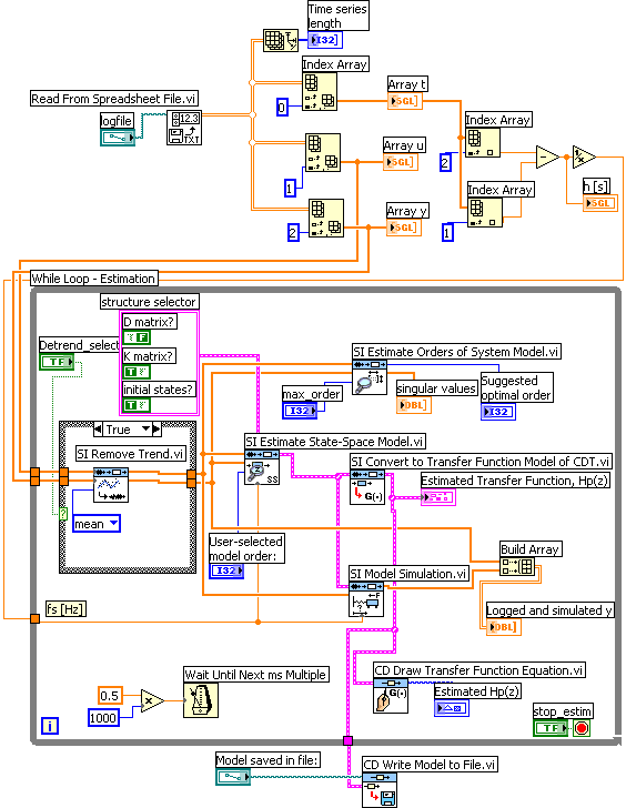
When a models is accurate, a control system can be designed and/or analyzed using the model.

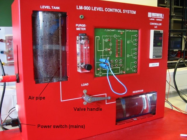
Water tank

[Contents]

5 Simulation of physical processes and its control system

Example: Simulation of a ship dynamic positioning system

At Buskerud University College students implement a simulator of a ship dynamic positioning system in LabVIEW Simulation Module:

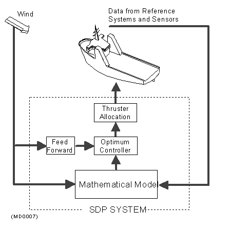
Ship dynamic positioning system

To limit the task, only the surge position is simulated:

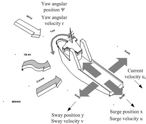
Motion coordinates of a ship

We have got real parameter values of a test ship from Konsberg Maritime. The model is as follows  (only the first of the three differential equations is considered):

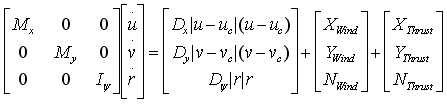
Mathematical model of ship

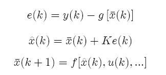
A PID controller is implemented. The controller includes feedforward from estimated water current (uc) which is estimated by a Kalman Filter. The inbuilt PID Advanced function is used. The Kalman Filer is implemented in Formula node. The Kalman Filter gain is calculated used the Kalman Gain function of Control Design Toolkit.

The Kalman Filter equations:

[Contents]

Example: Simulation of a clutch servo

Students at Buskerud University College implement a simulator of a clutch positional servo based on a mathematical model given by Konsberg Automotive. The mathematical model to be implemented in LabVIEW Simulation Module is as follows:

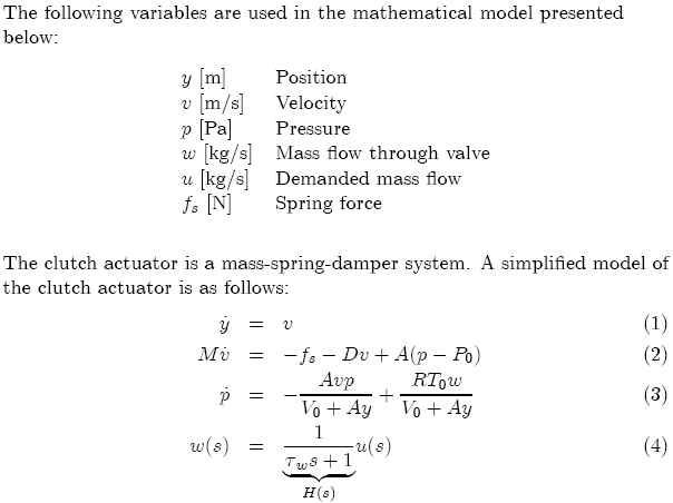
Below is the front panel of one implementation:

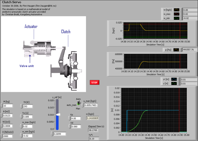
Front panel of the clutch servo simulator

[Contents]

6 State estimation using Kalman Filter algorithm

Example: The load torque of a DC motor is estimated with a Kalman Filter

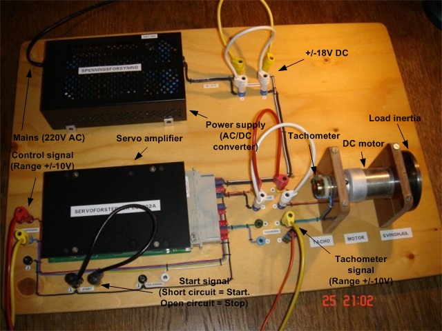
DC motor

The underlying mathematical model:

y=[1/(T*s+1)]*(K*u + L)

where y is tachometer voltage, u is control voltage, and is load torque (in equivalent voltage). K is the gain, and T is the time constant.

An equivalent state-space model: Define x₁ = y, and x₂ = L. Assuming that x₂ = L is (almost) constant, the model becomes

T*dx₁/dt = -x₁ + K*u + x₂

dx₂/dt = 0

y = x₁

The Kalman Filter equations: General form:

In our example, using the Euler forward method for discretization, the Kalman Filter equations are:

e = y - xpri1;

xpost1 = xp1 + k1*e;
xpost2 = xp2 + k2*e;

xpri1 = (1-(Ts/T))*xpost1 + (Ts/T)*xpost2 + (K*Ts/T)*uk;
xpri2 = xpost2;

These equations are implemented in a Fromula Node. The Kalman Filter gain is calculated used the Kalman Gain function of Control Design Toolkit.

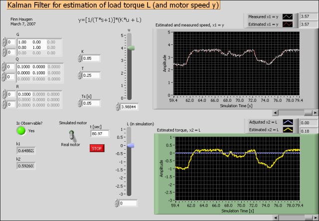
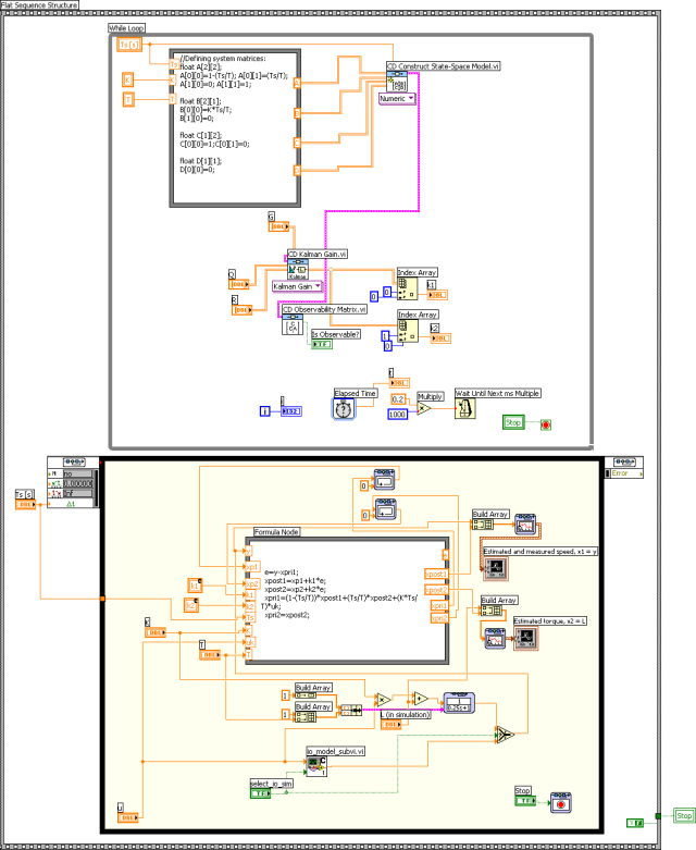
Front panel and block diagram of kalmanfilter_dcmotor_usb_io_sim.vi

Demo: kalmanfilter_dcmotor_usb_io_sim.vi.

In the above application two files are involved. They are zipped into this file: kalmanfilter_dcmotor_usb_io_sim.zip

[Contents]

March 16, 2007. By Finn Haugen, Associate Professor at Telemark University College. Also working in TechTeach. E-mail: finn@techteach.no.