|
|
|
Introduction to
LabVIEW Control Design Toolkit
1.0
by
Finn Haugen
January 30, 2005
Freeware!
Contents:
1 Preface
2 The contents of the Control Design Palette
3 Creating models
3.1 Creating
continuous-time (s-)transfer functions
3.2 Creating
discrete-time (z-)transfer functions
3.3 Creating
continuous-time state-space models
3.4 Creating
discrete-time state-space models
3.5 Standard
transfer functions
3.6 PID
controllers
3.7 Writing
models to file. Reading models from file
3.8 Getting
information about a model
3.9 Converting
Control Design models to/from Simulation Module models
4 Connecting models
4.1 Series
connection
4.2 Feedback
connection
5 Calculating transfer
functions from state-space models
6 Discretizing continuous-time models
7 Simulation (time
responses)
8 Frequency response
9 An application: Control
system analysis and simulation
1 Preface
This document gives an introduction to the Control Design Toolkit version 2.0 for LabVIEW 7.1. (LabVIEW is produced by National Instruments.) It is assumed that you have basic knowledge about LabVIEW programming.
The introduction is based on simple examples - all downloadable via hyperlinks. Only the basic functions are demonstrated. You can search for a function via the Help menu in LabVIEW or just browse for it on the Control Design palette in the Functions palette in LabVIEW. Chapter 2 of this document list all functions available in the Control Design Toolkit.
Each function has several input parameters or arguments. You should always use Help (via right-clicking on the function block) to get information about these parameters before you use the function in your program.
The Control Design Toolkit was initially launched in Spring 2004. It expands LabVIEW's capabilities for control system and dynamic system analysis and design considerably. The set of functions available is comparable with the Control System Toolbox in Matlab and the similar control system function category in Octave.
Included in version 2.0 is the Control Design Assistant, which is an interactive tool which can be used independent of LabVIEW, and without LabVIEW programming (you can however create LabVIEW code from your Control Design Assistant project). The Control Design Assistant is available from the Start / Programs / National Instruments meny on your PC and from the Tools / Control Design Toolkit in LabVIEW.
The VIs in the examples does not contain any while loops. Consequently, the VIs run just once. If you want a VI to run continuously with a well-defined time step between each while loop execution, possibly while you are adjusting some parameters, you can place the block diagram code in while loop.
If you have comments or suggestions for this document please send them via e-mail to finn@techteach.no.
In the text, CDT will be used as an abbreviation for Control Design Toolkit.
The date shown in the beginning of the document indicates the version of the document. The document may be updated any time. Changes from previous versions will be described in the Preface.
2 The contents of the Control Design Palette
Once the Control Design Toolkit is installed, the Control Design palette is available from the Functions palette. The Control Design palette is shown in the figure below.
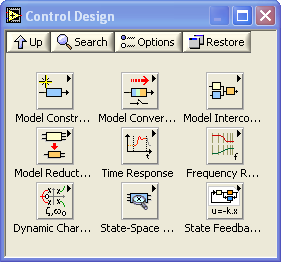
The Control Design palette
Below is a list of functions (and possible subpalettes) on the Control Design palette. (It may be wise to just browse the list to get a quick impression of the possibilities.)
- The Model Construction palette, with the following functions
and/or subpalettes:
- Construct State-Space Model
- Construct Transfer Function Model
- Construct Zero-Pole-Gain Model
- Construct Random Model
- Construct Special Model:
- First order with (or without) time delay
- Second order with (or without) time delay
- Delay Pade Approximation
- PID Parallel
- PID Academic (parallel form)
- PID Serial
- Draw Transfer Function Equation (for displaying the transfer function nicely on the screen, as writing on paper)
- Draw Zero-Pole-Gain Equation
- Read Model From File
- Write Model From File
- Model Information palette (containing functions for setting and getting model information or properties)
- The Model Conversion palette, with the following functions:
- Convert to State-Space Model
- Convert to Transfer Function Model
- Convert to Zero-Pole-Gain Model
- Convert Delay with Pade Approximation
- Convert Delay to Poles at Origin
- Convert Continuous to Discrete (with various methods, e.g. Euler, Tustin, zero order hold)
- Convert Discrete to Discrete (changing the sampling interval)
- Convert Discrete to Continuous
- Convert Control Design to Simulation (converting models used in Control Design Tookit for use in Simulation Module)
- Convert Simulation to Control Design (converting models used in Simulation Module for use in Control Design Tookit)
- The Model Interconnection palette, with the following
functions and/or subpalettes:
- Serial
- Parallell
- Feedback
- Append
- Rational Polynomial palette with functions for combining polynomials
- The Model Reduction palette, with the following functions:
- Minimal Realization
- Model Order Reduction
- Minimal State Realization
- Remove IO (input or output) from Model
- Select IO (input or output) from Model
- The Time Response palette, with the following functions
and/or subpalettes:
- Step Response (step input)
- Impulse Response (impulse input)
- Initial Response (response from initial state, with zero input)
- Linear Simulation (with user-defined input signal)
- Get Time Response Data
- The Frequency Response palette, with the following functions:
- Bode (calculating frequency response data and plotting the data in a Bode diagram)
- Nyquist
- Nichols
- Singular Values
- All Margins
- Gain and Phase Margin
- Evaluate at Frequency
- Bandwidth
- Get Frequency Response Data
- The Dynamic Characteristics palette, with the following
functions:
- Root Locus
- Pole-Zero Map
- Damping Ratio and Natural Frequency
- DC Gain
- Stability
- Norm
- Covariance Response
- Total Delay
- Distribute Delay
- Parametric Time Response
- The State Space Model Analysis palette, with the following
functions:
- Controllability Matrix
- Observability Matrix
- Grammians
- Canonical State-Space Realization
- Balance State-Space Model (Diagonal)
- Balance State-Space Model (Grammians)
- Controllability Staircase
- Observability Staircase
- State Similarity Transform
- The State Feedback Design palette, with the following
functions:
- Ackermann
- Pole Placement
- Linear Quadratic Regulator
- Kalman Gain
- State Estimator
- State-Space Controller
- Augment Output with States
3 Creating models
3.1 Creating and displaying continuous-time (s-)transfer functions
The Model Construction palette contains several functions for creating models. The resulting model is represented as a cluster. This cluster can be used as input argument to other functions, e.g. for simulation, frequency response analysis, etc.
On the Model Construction palette there are also functions for displaying the transfer function nicely on the front panel.
Example 3.1.1: Creating and displaying a continuous-time (s-)transfer function
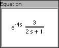
The VI shown below creates the following transfer function using the CD Construct Transfer Function Model function (CD means Control Design):
H(s) = e-4s 3/(1+2s) = e-4s 3s0/(1s0+2s1)
(a first order transfer function with gain 3, time constant 2, and time delay 4s). In the VI the CD Draw Transfer Function function displays the transfer function nicely in on the front panel (using a picture indicator which can be created by right-clicking on the Equation output of the function).
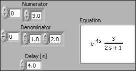
Front panel and block diagram of create_tf_cont.vi.
End of Example
Note: If the time delay is zero, the Delay input argument of the CD Construct Transfer Function Model function can be unwired since the default value of the time delay is zero.
Also note: The CD Construct Transfer Function Model function has an input parameter called Sampling Time. When creating continuous-time models this input must be either unwired (as in Example 3.1) or wired with value zero. If a non-zero sampling time is connected, a discrete-time transfer function will be created (with the numerator and denominator coefficients as defined in the Numerator and Denominator arrays). Cf. Section 3.2.
3.2 Creating discrete-time (z-)transfer functions
Example 3.2.1: Creating a discrete-time (z-)transfer function
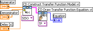
The VI shown below creates the following transfer function:
H(z) = z-5 0.4/(-0.6+z) = z-5 0.4z0/(-0.6z0+1z1)
with sampling time 0.1s. The factor z-5 represents a time delay of integer 5 samples (or time steps), not 5 seconds. (For the present transfer function, the time delay in seconds is 0.1*5 = 0.5s.)
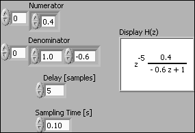
Front panel and block diagram of create_tf_discrete.vi.
End of Example
3.3 Creating continuous-time state-space models
Example 3.3.1: Creating a continuous-time state-space model
The VI shown below creates the following continuous-time state-space model using the CD Construct State-Space Model function:
In the VI the matrices are represented by arrays. For all models (no matter the order or dimension of the system) these arrays are 2-dimensional arrays.
Front panel and block diagram of create_cont_ss_model.vi.
End of Example
Note: The CD Construct State-Space Model function has an input parameter called Sampling Time. When creating continuous-time models this input must be either unwired (as in Example 3.3) or wired with value zero. If a non-zero sampling time is connected, a discrete-time state-space model will be created (with the system matrices as defined by the 2-dimensional arrays A, B, C, and D).
3.4 Creating discrete-time state-space models
Example 3.4.1: Creating a discrete-time state-space model
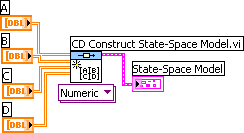
The VI shown below creates the following discrete-time state-space model using the CD Construct State-Space Model function:
x(k+1) = Ax(k) + Bu(k)
y(k) = Cx(k) + Du(k)
where the system matrices A, B, C, and D are as shown in the figure below. In the VI the matrices are represented by arrays. Note that the matrices are technically 2x2 matrices (arrays), although there may be only one row and/or column in the matrix.
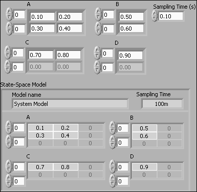
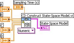
Front panel and block diagram of create_discrete_ss_model.vi.
End of Example
3.5 Standard transfer functions
Several standard transfer functions are available:
- First order with (or without) time delay
- Second order with (or without) time delay
- Delay Pade Approximation
Example 3.5.1: First order system with time delay
The VI below creates a first order transfer function with gain 2, time constant 3 seconds and time delay 4 seconds.
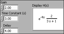
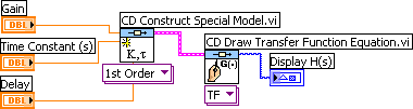
Front panel and block diagram of first_order_with_time_delay.vi.
End of Example
3.6 PID controllers
Several verions of PID controls are available as transfer functions:
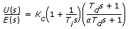
- PID Academic:
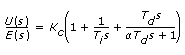
-
PID Parallel:
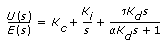
-
PID Serial:
Example 3.6.1: PID controller
The VI shown below shows how to create and display an PID Academic controller (which is a standard parallel PID controller). (The derivative time is set to zero, so the controller is actually a PI controller.)
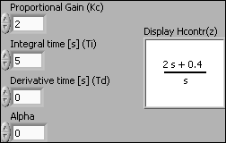
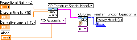
Front panel and block diagram of pid_controllers.vi.
End of Example
3.7 Writing models to file. Reading models from file
Models can be written to a file, and later read from that file, using the CD Write Model to File and CD Read Model from File functions, respectively.
Example 3.7.1: Writing a transfer function model to a file
The VI shown below shows how to write a transfer function model to a file.
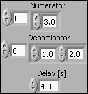
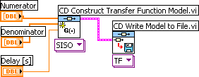
Front panel and block diagram of file_write_model.vi.
When the CD Write Model to File function is executed the usual Save File dialog window appears. (If you have wired a file path to the File Path input of the function, this dialog window is not opened.) You can give the file any name (the file extension does not matter).
End of Example
A model can be read from a model file using the CD Read Model from File function.
Example 3.7.2: Reading a transfer function model from a file
The VI shown below shows how to read a transfer function model from a file. (The model is the same as in Example 3.7.1.)
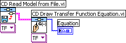
Front panel and block diagram of file_read_model.vi.
When the CD Read Model from File function is executed a File dialog window appears. (If you have wired a file path to the File Path input of the function, this dialog window is not opened.)
End of Example
3.8 Getting information about a model
You can get various information about a model by using functions on the Create Model / Model Information subpalette.
Example 3.8.1: Getting the numerator and denominator coeffiecient arrays of a transfer function model
The VI shown below shows how to get the numerator and denominator coeffiecient arrays of a transfer function model using the CD Get Data from Model function.
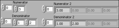
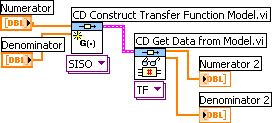
Front panel and block diagram of get_model_data.vi.
End of Example
3.9 Converting Control Design models to/from Simulation Module models
You can use models created in Control Design Toolkit in a Simulation diagram in the LabVIEW Simulation Module. However, it is then necessary to first convert the model by using the CD Convert Control Design to Simulation function.
Example 3.9.1: Converting a Control Design Toolkit model to a Simulation Module model
The VI shown below shows how to convert a transfer function model.
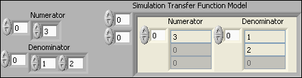
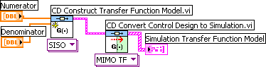
Front panel and block diagram of convert_to_simmodule.vi.
End of Example
4 Connecting models
The Model Interconnection palette contains several functions for connecting models. Series connection and a feedback connection of transfer functions are described in the following.
4.1 Series connection
Example 4.1.1: Series connection of transfer function models
The VI shown below shows how to get the resulting transfer function of two transfer functions connected in series using the CD Series function.
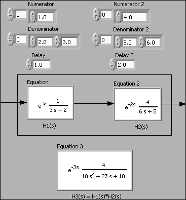
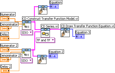
Front panel and block diagram of serial_connection.vi.
End of Example
4.2 Feedback connection
In models of feedback control systems, transfer functions are connected in a feedback loop. The resulting transfer function can be calculated using the CD Feedback function. This functions works for continuous-time models and for discrete-time models.
Example 4.2.1: Feedback connection of continuous-time transfer function models
The VI shown below shows how to get the resulting transfer function of two continuous-time transfer functions connected in a feedback loop.
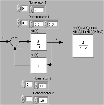
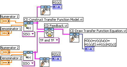
Front panel and block diagram of feedback_connection.vi.
End of Example
Note: For continuous-time models, the CD Feedback function ignores a time delay included in any of the transfer functions in the feedback loop, that is, the resulting transfer function is derived assuming the time delays are zero. To actually include the time delay(s), use the CD Construct Special Model function with the option Delay (Pade Approx.) selected to create a rational transfer function representing (and approximating) the time delay. Then include this transfer function in the feedback loop using e.g. the CD Series function. This is demonstrated in Example 9.1.
The following example shows how to connect discrete-time transfer functions including time delays in a feedback loop. It is necessary to convert the time delay part of a discrete-time model to poles at the origin using the CD Convert Delay to Poles at Origin function for the CD Feedback function to produce the correct transfer function of the combined feedback loop. This also applies to discrete-time transfer functions which have been derived by discretizing an original continuous-time transfer function, that is, you have to use the CD Convert Delay to Poles at Origin function for the CD Feedback function to produce the correct result.
Example 4.2.2: Feedback connection of discrete-time transfer function models including time delay
In the VI shown below two discrete-time transfer functions are connected in a feedback loop. One of the transfer functions, H2(z), contains a time delay of 2 samples, corresponding to 2 poles at the origin of the z-plane.
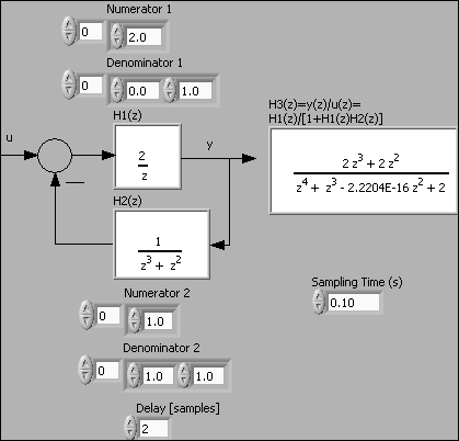
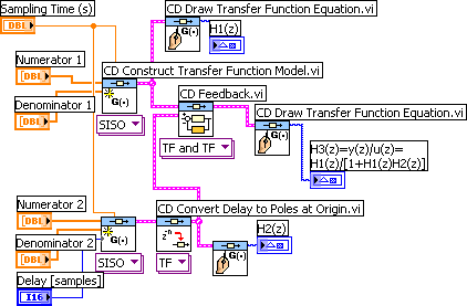
Front panel and block diagram of feedback_connection_discrete.vi.
End of Example
5 Calculating transfer functions from state-space models
The CD Convert to Transfer Function Model function converts continuous-time and discrete-time state-space models to transfer function models. The resulting transfer function model is actually a MIMO (multiple input multiple output) transfer function, i.e. a transfer function matrix. To get a particular SISO (single input single output) transfer function from this MIMO transfer function you must apply the CD Get Data from Model function. This is illustrated in the following example. This example is about a continuous-time model, but the same functions are used for discrete-time models.
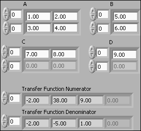
Example 5.1: Calculating transfer function from state-space model
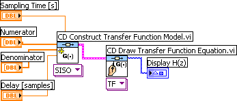
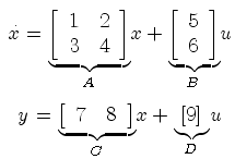
The VI shown below shows how to get the SISO transfer function from input u to output y from the state-space model
dx/dt = Ax + Bu
y = Cx + Du
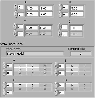
where the system matrices are as shown on the VI front panel below.
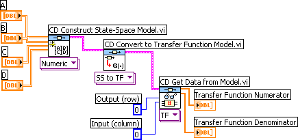
Front panel and block diagram of convert_ss_to_tf.vi.
Note that the indexing of the rows and the columns start with indices 0, i.e. the first row has index 0, and the first column has index 0.
End of Example
6 Discretizing continuous-time models
The following example illustrates how to discretize a continuous-time transfer function using the CD Convert Continuous to Discrete function. The same function can be used to discretize state-space models. Converting a model the opposite way - from discrete-time to continuous-time - is done in a similar way using the CD Convert Discrete to Continuous function.
Example 6.1: Discretizing a continuous-time transfer function
The VI shown below shows how to do the discretization using the ZOH method (zero order hold) with sampling time 0.2s. The original transfer function contains a time delay of 1 second. This time delay is represented in the discrete-time transfer function by the factor z-5 (since 5*0.2s = 1s).
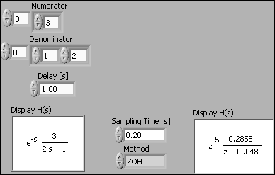
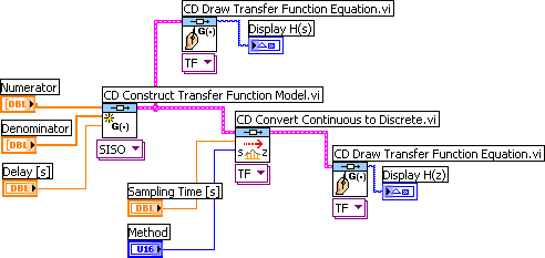
Front panel and block diagram of convert_cont_to_discrete.vi.
End of Example
7 Simulation (time responses)
The Time Response palette contains several simulation functions for simulating step response, impulse response, arbitrary input response, and initial state response. The following example shows how to simulate the step response.
The simulations are run as a "batch" simulation, being completed as fast as the PC allows. If you want a real-time simulation, i.e. the simulation develops along a real time axis, you can use LabVIEW Simulation Module. Models created in the Control Design Toolkit can be used in the Simulation Module by using the models conversion functions demonstrated in Chapter 3.10.
Example 7.1: Simulation of the step response of a continuous-time transfer function
The VI shown below simulates the step response of the following transfer function:
H(s) = 3/(1+2s)
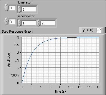
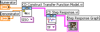
Front panel and block diagram of step_response_tf_model.vi.
CD Step Response simulates with a unity step (amplitude 1) at the model input.
The graph indicator can be created by right-clicking on the Step Response Graph output of the CD Step Response function.
End of Example
8 Frequency response
The Frequency Response palette contains several functions for generating and plotting frequency response data - for continuous-time as well as discrete-time models.
Example 8.1: Frequency response of a continuous-time transfer function
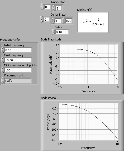
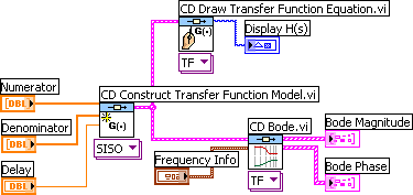
Front panel and block diagram of frequency_response.vi.
End of Example
9 An application: Analysis and simulation of control system
Example 9.1: Control system analysis and simulation
The VI shown below shows how to analyze and simulate a feedback control system. The block diagram code is put inside a while loop with cycle time 100ms to make the program run continuously. The controller is a PID Academic controller (which has parallel form) with the following transfer function, Hc(s):
A Pade approximation is used to represent the time delay of the process because the CD Feedback function works correctly only if there are only rational transfer functions in the feedback loop.
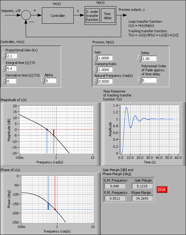
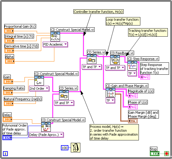
Front panel and block diagram of controlsys_analysis.vi.
End of Example
More free stuff from TechTeach:
- KYBSIM - free simulators, ready to run!
- Introduction to LabVIEW Simulation Module
- Introduction to discrete-time signals and systems